Reading for Lab #4 on Mon., Feb 14:
PDF version
Instructions for Lab #4: Convection and Clouds
Note:
Something to note:
- One big piece of this lab is to use RMarkdown to write a report that really integrates text with code and graphics and tables that are generated by RMarkdown. Use the fact that you can easily check your answers to the specific questions to give you some freedom to think about how you want to present your answers. Don’t just copy and paste from my answers, but think about how you would use RMarkdown to present your answers in your own way.
Exercises with lapse rate and clouds.
In this lab, you will learn about a new climate model, RRTM. RRTM stands for “Rapid Radiative Transfer Model.” This model is a radiative-convective model that uses code from the radiative-transfer portion of a state-of-the-art global climate model called the “Community Earth System Model,” developed at the National Center for Atmospheric Research in Boulder CO.
The entire CESM model runs on giant supercomputers, but this radiative transfer module can run efficiently on an ordinary computer. In order to speed up the calculations, RRTM does not calculate the entire longwave spectrum the way MODTRAN does, but uses a simplified approximation that is much faster when the big climate models need to run this radiative transfer calculation roughly 52 quadrillion (5.2×10¹⁵) times in a simulation of 100 years of the earth’s climate.
An advantage that RRTM has over MODTRAN, is that MODTRAN assumes that the atmosphere is static (none of the air moves), whereas RRTM allows for convective heat flow. This makes RRTM more realistic, even though it sacrifices detail in its treatment of longwave radiation.
We will use RRTM to explore the role of convection in the earth system and to examine the water-vapor feedback in the presence of convection.
You can run the RRTM model interactively on the web at http://climatemodels.uchicago.edu/rrtm/ and I have also written a script that allows you to run it from R.
To run the model interactively, you can adjust various parameters, such as the brightness of the sun, the albedo (it gives you a choice of many natural and human-made surfaces, such as asphalt, concrete, forest, grassland, snow, ocean, and the average for the earth) the concentrations of CO2 and methane, the relative humidity, and the amount and type of high (cirrus) and low (stratus) clouds.
You can also introduce aerosols typical of different parts of the earth, such as cities (with soot, sulfates, and other pollution), deserts (with blowing dust), oceans (with sea spray and salt), and a Pinatubo-like volcanic eruption.
Like MODTRAN, the RRTM model does not automatically adjust the surface temperature. Instead, it calculates the upward and downward flux of longwave and shortwave radiation at 51 different levels of the atmosphere and reports whether the heat flow is balanced (heat in = heat out) at the top of the atmosphere.
If the earth is gaining heat, you can manually raise the surface temperature until you balance the heat flow, and if the earth is losing heat, you can manually lower the temperature.
R Interface to RRTM
I have written an R function run_rrtm that allows you to manually run
RRTM from R. To use this function, you need to include the line
source("_scripts/rrtm.R") or source(file.path(script_dir, "rrtm.R"))
to load it.
run_rrtm()allows you to automatically download a file with the data from a MODTRAN run. You call it with the following arguments:filenameis the name of the file to save the data to. The function returns the output data, so it’s optional to specify a file name.co2_ppmis the amount of CO2 in parts per million. The default is 400.ch4_ppmis the amount of methane in parts per million. The default is 1.7.relative_humidityis the relative humidity, in percent. The default is 80%.T_surfaceis the surface temperature, in Kelvin. The default (for 400 ppm CO2, etc.) is 284.42. You adjust this to restore radiative equilibrium after you change the parameters (amount of CO2, lapse rate, etc.).I_solaris the brightness of the sun, in Watts per square meter. The default value is 1360.surface_typeis the type of surface (this is used to calculate the albedo). The default is `earth average. The options are:- “
earth average”: The average albedo of the earth (0.30) - “
asphalt”: Dark asphalt (0.08) - “
concrete”: Concrete (0.55) - “
desert”: Typical desert (0.40) - “
forest”: Typical forest (0.15) - “
grass”: Typical grassland (0.25) - “
ocean”: Ocean (0.10) - “
snow”: Typical snow (0.85) - “
ice”: Large ice masses covering ocean or land (0.60) - “
soil”: Bare soil (0.17) - “
custom”: Custom albedo (if you choose this, you need to also supply a value foralbedo)
- “
tropopause_kmis the altitude of the tropopause, in kilometers above sea level. The default value is 15, which is typical of middle latitudes. The tropopause varies from place to place around the Earth, from around 9 km at the poles to around 17 km near the equator.lapse_rateis the lapse rate, in Kelvin per kilometer. The default is 6, which is roughly the global average environmental lapse rate. The dry adiabatic lapse rate is 10, so it’s physically impossible to have an persistent environmental lapse rate greater than 10 and results withlapse_rategreater than 10 won’t make sense.low_cloud_fracis the fraction (from 0.0–1.0) of the sky covered by low (stratus) clouds. The default is 0.0.high_cloud_fracis the fraction (from 0.0–1.0) of the sky covered by high (cirrus) clouds. The default is 0.0.cloud_drop_radiusis the size of the water droplets in the clouds, in microns. The default is 10. (For reference, 10 microns is about the size of a red blood cell). You can make the droplets smaller to simulate the indirect aerosol effect.aerosolsallows you to set up the atmosphere with the kinds and quantities of aerosols typical of a number of different environments. Options are:- “
none”: No aerosols - “
ocean”: Typical ocean aerosols (sea-spray, salt, etc.) - “
desert”: Typical desert aerosols (dust, sand) - “
city”: Typical city with soot (black carbon) and sulfate aerosols. - “
city just sulfates”: Just sulfate aerosols typical of a city. - “
city just soot”: Just soot (black carbon) aerosols typical of a city. - “
land”: Typical rural land (dust, etc.) - “
polluted land”: Typical rural land suffering from pollution (e.g., from farming) - “
antarctic”: Typical aerosols for Antarctica - “
volcano”: Similar sulfate and dust to the Mt. Pinatubo volcanic eruption.
- “
Any arguments you don’t specify explicitly take on their default value. Thus,
run_rrtm(co2_ppm = 800, relative humidity = 10, T_surface = 300)would run with all the default values, except for 800 ppm CO2, relative humidity of 10%, and a surface temperature of 300 Kelvin.run_rrtmreturns a list of data containing:- Basic parameters of the model run:
T_surfaceco2_ppmch4_ppmI_solaralbedolapse_ratetropopause_kmrelative_humidityaerosols,low_cloud_frachigh_cloud_fraccloud_drop_radius
- Results of the model calculations:
Q: The heat imbalance \(I_{\text{in}} - I_{\text{out}}\)i_in: The net solar radiation absorbed by the earth (\((1 - \alpha) I_{\text{solar}} / 4\))i_out: The net longwave radiation emitted to space from the top of the atmosphereprofile: A tibble containing a profile of the atmosphere (altitude in km, pressure in millibar, and temperature in Kelvin)fluxes: A tibble containing the fluxes (in Watts per square meter) of longwave, shortwave, and total radiation going up and down at 52 levels from the surface to the top of the atmosphere. The columns arealtitude(km),T(temperature in K),P(pressure in millibar),sw_up(upward shortwave),sw_down(downward shortwave),lw_up(upward longwave),lw_down(downward longwave),total_up(sw_up+lw_up), andtotal_down (sw_down+lw_down`).
There are also functions for reading RRTM data files and plotting RRTM data:
read_rrtm(file)reads an RRTM file saved byrun_rrtmand returns a list of data just like the one returned byrun_rrtm.plot_heat_flows(): plots the upward and downward fluxes of radiation from an RRTM file or data structure. You can call it either withplot_rrtm(file = "filename")orplot_rrtm(data = rrtm_data), where “filename” and “rrtm_data” stand for your own file name or RRTM data structure returned byrun_rrtmorread_rrtm.You can also specify which wavelengths to plot. By default, it plots shortwave (SW), longwave (LW), and total (SW + LW), but you can specify one or more of
sw = FALSE,lw = FALSE, ortotal = FALSEto omit wavelengths.
Example of running RRTM
Here is an example of running RRTM:
default_rrtm = run_rrtm()

# Surface temperature:
default_rrtm$T_surface
## [1] 284.42# Heat imbalance:
default_rrtm$Q## [1] 0This run has surface temperature 284. K and a heat imbalance of 0 Watts per square meter.
Interpreting RRTM Results
We can plot the heat flows as a function of altitude:
plot_heat_flows(default_rrtm)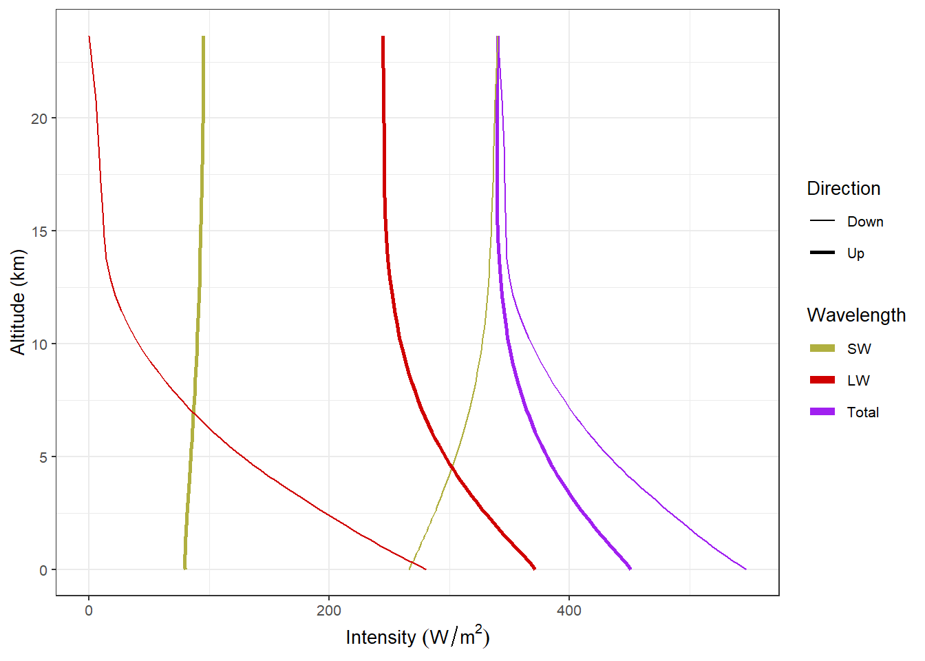
What you see in this plot are thick lines representing downward heat flow and thin lines representing upward flow. The different colors represent shortwave, longwave, and total (shortwave + longwave).
A few things to notice: At the top of the atmosphere, at 20. km, there is very little longwave going down, but a lot of shortwave going down (around 340. W/m2). Conversely, there is a modest amount of shortwave going up (around 100. W/m2), but a lot of longwave going up (around 240. W/m2).
The upward shortwave radiation is sunlight reflected from the atmosphere and the earth’s surface.
The upward longwave radiation is emitted from the surface and the atmosphere. You can see that the longwave radiation, both up and down, is greater closer to the surface, where temperatures are warmer, and smaller at higher altitudes, where the atmosphere is cooler.
If we look at the total radiation, we see that there is a good balance near the top of the atmosphere (the upward and downward lines come together), but in the lower atmosphere, there is a serious imbalance with downward fluxes significantly larger than the upward ones.
This is a consequence of convection: The difference between the downward and upward radiative fluxes is taken up by convection, which moves heat upward when warm air rises and cool air sinks.
Determining Climate Sensitivity with RRTM
We can also use the RRTM model to study what happens when we double CO2:
rrtm_double_co2 = run_rrtm(co2_ppm = 800)When we double CO2 without changing the surface temperature (Tsurface = 284.4 K), this creates a heat imbalance of 4.2 W/m2. We can use the online interactive version of RRTM to adjust surface temperature until the heat flows balance. The surface temperature where this happens is 286.9 K and we can paste it into our R code:
new_ts = 286.9 # Kelvin
rrtm_double_co2_balanced = run_rrtm(co2_ppm = 800, T_surface = new_ts)
When we set Tsurface to 286.9 K, the heat imbalance becomes 0 Watts/m2. The climate sensitivity is the change in equilibrium Tsurface when you double CO2: \(\Delta T_{2\times \text{CO}_2} = 286.9~\mathrm{K} - 284.4~\mathrm{K} = 2.5~\mathrm{K}\). You may remember that in last week’s lab, we calculated the climate sensitivity with MODTRAN (using constant relative humidity to enable water-vapor feedback) and got \(\Delta T_{2\times\text{CO}_2} = 1.2\) K for the tropical atmosphere (it’s smaller for the other atmospheres), so this shows that including convection in our calculations roughly doubles the climate sensitivity.
New R and RMarkdown tricks
Sometimes you may want to use different text into your document, depending on what the result of a calculation is.
For instance, I might have a function called foo that returns a number
and I want to write something different if foo(x) > x than if
foo(x) < x. Here, the function ifelse can come in handy.
foo = function(x) {
  x^2
}
Now I can write ifelse(foo(x) < x, "less than", "greater than").
The following RMarkdown text:
When x = 0.5, `foo(x)` is
`r x = 0.5; ifelse(foo(x) < x, "less than", "greater than")` x,
but when x = 2.0, `foo(x)` is
`r x = 2.0; ifelse(foo(x) < x, "less than", "greater than")` x.
becomes
When x = 0.5,
foo(x)is less than x, but when x = 2.0,foo(x)is greater than x.
You may have spotted a problem with the code above: What if foo(x) = x?
Then I need another ifelse:
ifelse(foo(x) < x, "less than", ifelse(foo(x) > x, "greater than", "equal to")).
This is cumbersome to type into your text, so you might want to write a function:
compare_f = function(f, x) {
  # f is a function
  # x is a number or a numeric variable
  result = f(x)
  ifelse(result < x, "less than",
         ifelse(result > x, "greater than",
                "equal to"))
}
Now I can just write compare_f(foo, x):
The following RMarkdown text:
When x = 0.5, `foo(x)` is `r compare_f(foo, 0.5)` x, but
when x = 2.0, `foo(x)` is `r compare_f(foo, 2.0)` x, and
when x = 1.0, `foo(x)` is `r compare_f(foo, 1.0)` x.
becomes
When x = 0.5,
foo(x)is less than x, but when x = 2.0,foo(x)is greater than x, and when x = 1.0,foo(x)is equal to x.
This may seem kind of strange, but a lot of people and organizations use
RMarkdown to prepare reports regularly using different data.
For instance, many businesses use RMarkdown to generate monthly reports
on sales, finances, etc., and using code like the compare function I
showed here can help to automate the reports, so that when they run the
report each month using different data, the text will adjust automatically to
reflect the new numbers.
It is also applicable to climate science, where many laboratories like to update their reports every month or every year with the latest climate data.
Exercises
These are the exercises you will work for the lab this week.
General Instructions
In the past three weeks, we focused on mastering many of the basics of using R and RMarkdown. For this week’s lab, when you write up the answers, I would like you to think about integrating your R code chunks with your text.
For instance, you can describe what you’re going to do to answer the question, and then for each step, after you describe what you’re going to do in that step, you can include an R code chunk to do what you just described, and then the subsequent text can either discuss the results of what you just did or describe what the next step of the analysis will do.
This way, your answer can have several small chunks of R code that build on each other and follow the flow of your text.
For this lab, you will use the RRTM model, which includes both radiation and convection.
Exercise 1: Lapse Rate
Run the RRTM model in its default configuration and then vary the lapse rate
from 0 to 10 K/km. For each value of the lapse rate, adjust the surface
temperature until the earth loses as much heat as it gains (i.e., the value of
Q in the run_rrtm model output is zero.)
It will probably be easier to do this with the interactive version of the RRTM
model at http://climatemodels.uchicago.edu/rrtm/ than with the R interface
run_rrtm.
- Make a tibble containing the values of the lapse rate and the corresponding
equilibrium surface temperature, and then (in your report):
- Make a table showing lapse rate and temperature.
- Make a plot with lapse rate on the horizontal axis and surface temperature on the vertical axis.
- Describe how the equilibrium surface temperature varies as the lapse rate varies.
Exercises on Albedo and Clouds
For the following exercises, start off with the RRTM model in its default configuration. Record the ground temperature. For each part of this exercise you will do the following:
You will adjust the albedo or the clouds.
You will compare the visible and longwave radiation going down through the atmosphere to the surface and also the visible and longwave radiation going up from the surface, through the atmosphere, to space.
The results of an RRTM model run have a tibble called
fluxeswith columns foraltitude,sw_down,sw_up,lw_down,lw_up,total_down, andtotal_up, whereswmeans shortwave,lwmeans longwave, andtotalis the sum of shortwave plus longwave.The first row of this tibble is at ground-level and the last row is at the top of the atmosphere.
default_data = run_rrtm()
fluxes = default_data$fluxes
surface_fluxes = head(fluxes, 1) # get the first row
space_fluxes = tail(fluxes, 1)   # get the last row
You will adjust the ground temperature until the heat coming in balances the heat going out (the model will say, “If the Earth has these properties … then it loses as much energy as it gains.”
Exercise 2: The urban heat island
First, run the RRTM model in its default configuration and note the surface temperature and the albedo.
default = run_rrtm()
albedo_default = default$albedo
T_surface_default = default$T_surface
Change the surface type from “Earth’s average” to “Asphalt” (don’t change the surface temperature until the instructions tell you to) and describe the changes in the local climate:
- What is the albedo?
- Report the changes in shortwave and longwave light absorbed by the surface and going out to space.
- How much does the total balance of heat change (i.e., how many W/m2 does the Earth lose or gain)?
- Now, adjust the ground temperature until the Earth loses as much energy as it gains.
- What is the new surface temperature? How does it compare to the surface temperature in the default configuration?
Change the surface albedo to “Concrete”. Answer the same questions as in part (a).
In cities, streets and parking lots are usually paved with asphalt. Roofs of houses and other buildings are often covered with asphalt shingles or black rubber-like compounds.
The results you got in this exercise represent covering the entire planet with asphalt or concrete, so they are far more extreme than you would get from only covering part of a city with one material or the other, but the general principle holds and in a city you would have much smaller changes, but they would be in the same direction as you found here.
How would the choice of using asphalt for roads, parking lots, and roofs in a large city affect the local climate in the city? Would using low-albedo materials, such as concrete for streets and parking lots and light-colored polymers for the roofs of buildings have a benefit for the people living in the city?
Exercise 3: Clouds
First, run the RRTM model in its default configuration and note the surface temperature and the albedo.
Change the low cloud fraction to 0.70 (70%)
- Report the changes in shortwave and longwave light absorbed by the surface and going out to space.
- How much does the total balance of heat change (i.e., how many W/m2 does the Earth lose or gain)?
- Adjust the temperature to bring the heat flows back into balance.
- How much did the temperature change?
Repeat part (a), but with the low cloud fraction set to 0 and the high-cloud fraction set to 0.20 (20%).
Use the
plot_heat_flows()function to plot the heat flows for the low clouds and the high clouds. Describe the changes you see in the upward and downward heat flows (shortwave, longwave, and total) for the two cases. Which kind of cloud had the biggest effect on the outgoing radiation?
