Reading for Lab #6 on Mon., Feb 28:
PDF version
Instructions for Lab #6: The Carbon Cycle
Carbon Cycle
For the following exercises, you will use the GEOCARB model, which simulates the earth’s carbon cycle.
The GEOCARB model has two time periods:
First, it runs for 5 million years with the “Spinup” settings in order to bring the carbon cycle and climate into a steady state. Only the last 1000 years of the spinup are saved.
Then, at time zero, it abruptly changes the parameters to the “Simulation” settings and also dumps a “spike” of CO2 into the atmosphere and runs for another 2 million years with the new parameters to see how the climate and carbon cycle adjust to the new parameters and the CO2 spike.
The quantities that are graphed in the online version of the model include:
pCO2- is the concentration of CO2 in the atmosphere, in parts per million.
WeatC- is the rate of CO2 being weathered from carbonate rocks and moved to the
oceans.
BurC- is the rate of carbonate being converted into limestone and buried on the
ocean floor.
WeatS- is the rate of SiO2 being weathered from silicate rocks and moved to the
oceans.
Degas-
is the rate at which CO2 is released to the atmosphere by volcanic activity
tCO2- is the total amount of CO2 dissolved in the ocean, adding all of its forms:
\[ \ce{\text{tco2} = [CO2] + [H2CO3] + [HCO3-] + [CO3^{2-}]}. \]
alk- is the ocean alkalinity: the total amount of acid (\(\ce{H+}\)) necessary to
neutralize the carbonate and bicarbonate in the ocean. The detailed definition is complicated, but to a good approximation, \(\ce{\text{alk} = [HCO3-] + 2 [CO3^{2-}]}\). This is not crucial for this lab.
CO3- is the concentration of dissolved carbonate (\(\ce{CO3^{2-}}\)) in the ocean,
in moles per cubic meter.
d13Cocn- is the change in the fraction of the carbon-13 (\(\ce{^{13}C}\)) isotope,
relative to the more common carbon-12 (\(\ce{^{12}C}\)) isotope, in the various forms of carbon dissolved in the ocean water.
d13Catm- is the change in the fraction of \(\ce{^{13}C}\),
relative to \(\ce{^{12}C}\) in atmospheric CO2.
Tatm-
is the average air temperature.
Tocn- is the average temperature of ocean water.
Running the GEOCARB model from R
I have provided functions for running the GEOCARB model from R:
To run the model:
run_geocarb(co2_spike, filename, degas_spinup, degas_sim,
            plants_spinup, plants_sim, land_area_spinup, land_area_sim,
            delta_t2x, million_years_ago, mean_latitude_continents)
You need to specify co2_spike (the spike in CO2 at time zero, measured in
billions of tons of carbon).
The other parameters will take default values if you don’t specify them, but you can override those defaults by giving the parameters a value.
The arguments to the function are:
filename- an optional file to save the results of the run to. You can read them back
in using the read_geocarb() function:
r run_geocarb(spike = 1000, filename = "test_run.txt") data = read_geocarb("test_run.txt")
degas_spinupanddegas_sim- the rates of CO2 degassing from volcanoes for the spinup and simulation
phases, in trillions of molecules per year.
plants_spinupandplants_sim-
TRUEorFALSEvalues for whether to include the role of plants in
weathering (their roots speed up weathering by making soil more permeable
and by releasing CO2 into the soil), and land_area is the total area of
dry land, relative to today.
land_area_spinupandland_area_sim- The amount of land area, compared to today (1.0 means the same amount of
land as today).
delta_t2x- The climate sensitivity (the amount warming for each time CO2 is
doubled), in degrees Celsius.
million_years_ago- Simulate past climates when the sun was not as bright as today.
The value of this variable is how many million years ago the year zero of the simulation should be. This is not currently working because of a bug in the web version of GEOCARB.
mean_latitude_continents- The mean latitude, in degrees, of the continents.
The default values are: degas = 7.5, plants = TRUE, and land_area = 1
for both the spinup and the simulation.
The default value for delta_t2x is 3.0, million_years_ago is 0,
and mean_latitude_continents is 30, which corresponds to today’s world.
mean_latitude_continents and land_area allow you to explore conditions in
earth’s past, where the continents had different areas and were located in
different parts of the world.
million_years_ago is meant to allow you to explore how the silicate weathering
thermostat worked in earth’s past, when the sun was a lot less intense than it
is today. However, this part of the model is not working now.
After you run run_geocarb, you would read the data in with
read_geocarb(filename). This function will return a data frame with the columns
year, co2_total, co2_atmos, alkalinity_ocean,
delta_13C_ocean, delta_13C_atmos, carbonate_ocean,
carbonate_weathering, silicate_weathering, total_weathering,
carbon_burial, degassing_rate, temp_atmos, and temp_ocean.
Refresher on Plotting Several Variables
You may want to go back to the documentation for Lab #2 and refresh your
memory about the pivot_longer() function for manipulating data frames and
tibbles, and the different ways we can use ggplot to plot several variables
on the same plot.
Suppose you have a tibble with columns time, foo and bar,
as shown below:
df = tibble(time = seq(100), foo = -1 + 0.1 * time - 0.001 * time^2,
            bar = sin(time / 10))
kable(head(df), digits = 2)| time | foo | bar |
|---|---|---|
| 1 | -0.90 | 0.10 |
| 2 | -0.80 | 0.20 |
| 3 | -0.71 | 0.30 |
| 4 | -0.62 | 0.39 |
| 5 | -0.52 | 0.48 |
| 6 | -0.44 | 0.56 |
Now, suppose you want to plot foo and bar on the same graph.
You can do
ggplot(df, aes(x = time)) + geom_line(aes(y = foo), color = "darkred") +
geom_line(aes(y = bar), color = "darkblue")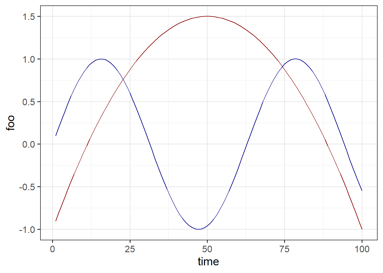 But it is more elegant to write
df_tidy = pivot_longer(df, cols = -time, names_to = "variable",
                       values_to = "value")
kable(head(df_tidy))| time | variable | value |
|---|---|---|
| 1 | foo | -0.9010000 |
| 1 | bar | 0.0998334 |
| 2 | foo | -0.8040000 |
| 2 | bar | 0.1986693 |
| 3 | foo | -0.7090000 |
| 3 | bar | 0.2955202 |
Now you can plot this:
ggplot(df_tidy, aes(x = time, y = value, color = variable)) + geom_line() +
         scale_color_manual(values = c(foo = "darkred", bar = "darkblue"))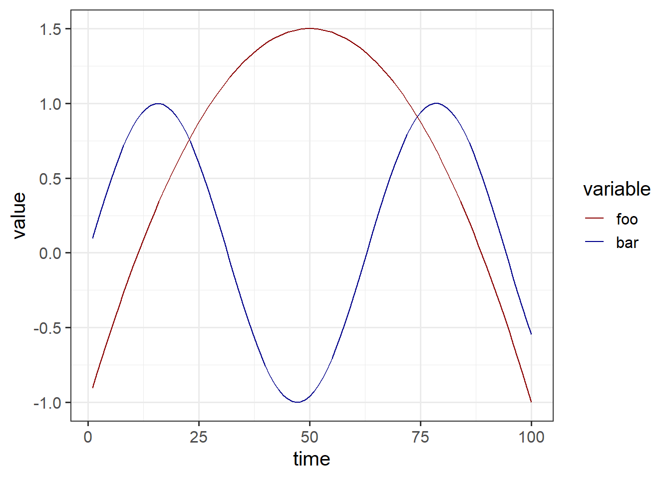
And you can put this all together in a single expression using pipes:
pivot_longer(df, cols = -time, names_to = "variable",
             values_to = "value") %>%
  ggplot(aes(x = time, y = value, color = variable)) + geom_line() +
  scale_color_manual(values = c(foo = "darkred", bar = "darkblue"))
Modifying the Axes of a Plot
Sometimes you have a lot of data and you just want to plot a small part of it. Consider the following GEOCARB model run:
geocarb_data = run_geocarb(1000)## Rows: 140 Columns: 14
## -- Column specification --------------------------------------------------------
## Delimiter: ","
## dbl (14): year, tco2, alk, d13Cocn, pCO2, d13Catm, CO3, WeatC, WeatS, TotW, ...
##
## i Use `spec()` to retrieve the full column specification for this data.
## i Specify the column types or set `show_col_types = FALSE` to quiet this message.ggplot(geocarb_data, aes(x = year, y = co2_atmos)) + geom_line() +
labs(x = "Year", y = "CO2")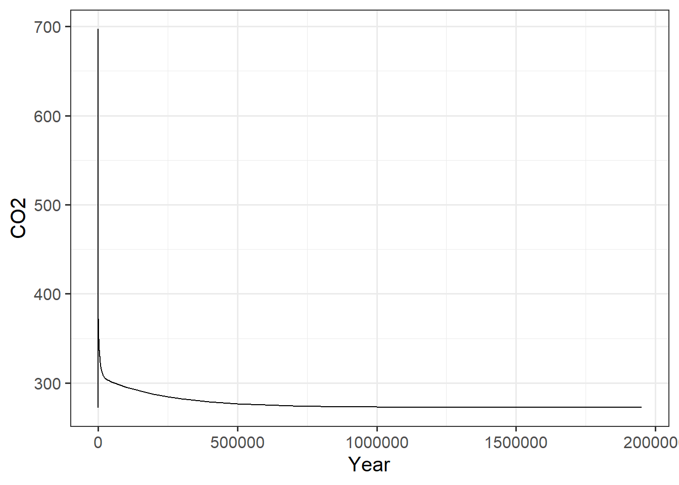
This shows us all 2 million years of the model run, but we can’t see the detail of what’s happening near year zero. There are several ways we can zoom our plot in to look only at the region near year zero:
Use the
xlimandylimfunctions to set limits:ggplot(geocarb_data, aes(x = year, y = co2_atmos)) + geom_line() + xlim(-500, 1000) + labs(x = "Year", y = "CO2")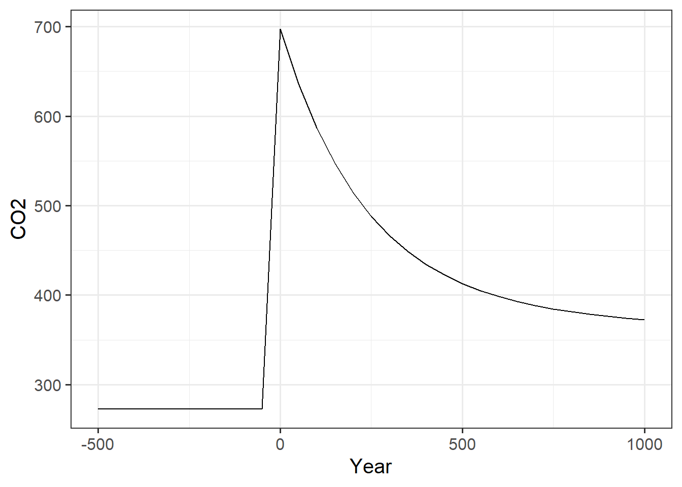
If you only want to change one limit, and leave the other at its default, you can put
NAfor the limit you want to leave alone:ggplot(geocarb_data, aes(x = year, y = co2_atmos)) + geom_line() + xlim(NA, 1000) + labs(x = "Year", y = "CO2")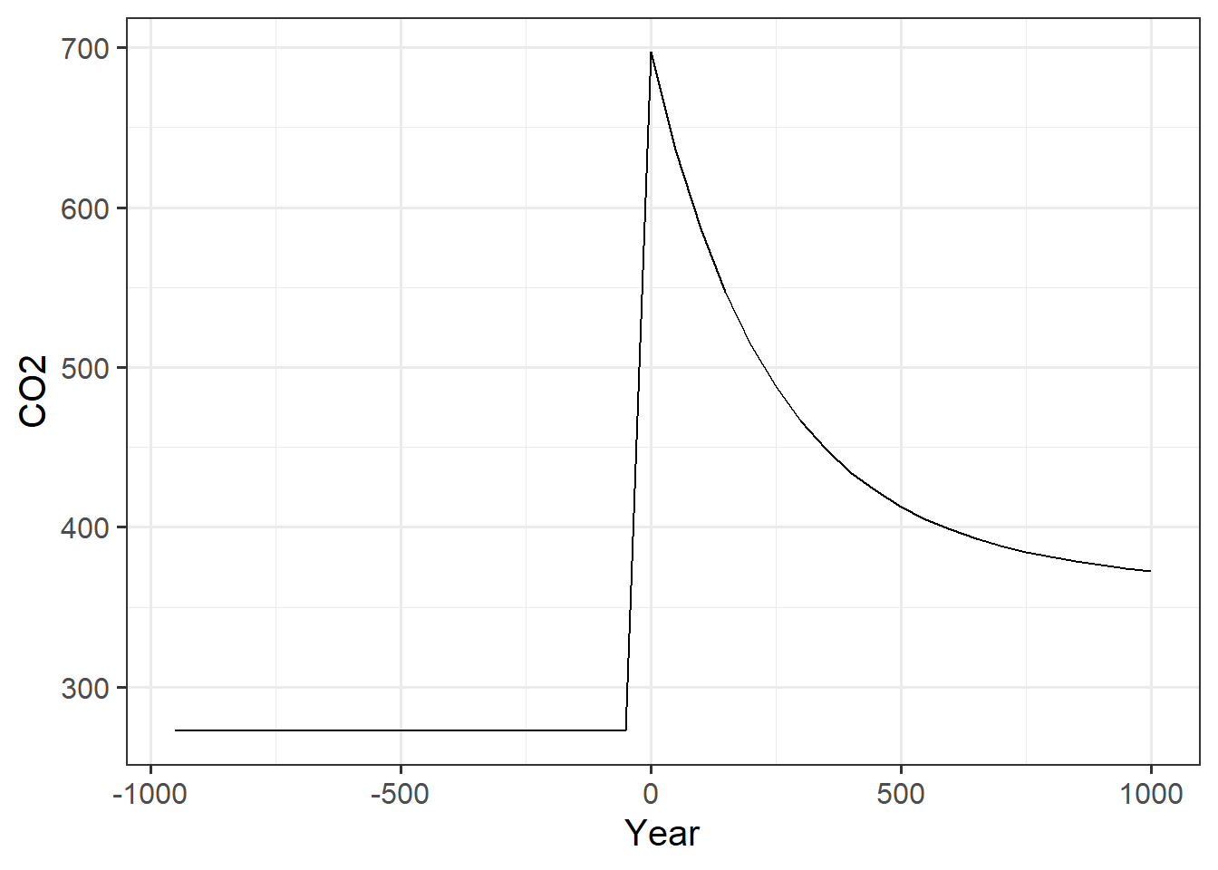
Use the
scale_x_continuousandscale_y_continuousfunctionsggplot(geocarb_data, aes(x = year, y = co2_atmos)) + geom_line() + scale_x_continuous(limits = c(NA, 1E4), labels = label_comma()) + labs(x = "Year", y = "CO2")
Using the
scale_x_continuousandscale_y_continuousfunctions lets you also modify the way numbers are formatted on the axis. Here, I used thelabel_comma()function to insert commas in the thousands and millions places. Other label commands includelabel_percent. You can read more about these at the web page for thescalespackage.Another approach to limiting the extent of the plot is to filter the data before you call
ggplotgeocarb_data %>% filter(year >= -500, year <= 1000) %>% ggplot(aes(x = year, y = co2_atmos)) + geom_line() + labs(x = "Year", y = "CO2")
Exercises for Lab #6
Exercise 1: Weathering as a Function of CO2
In the steady state, the rate of weathering must balance the rate of CO2 degassing from the Earth, from volcanoes and deep-sea vents.
Write this exercise up as a discussion of what happens when the rate of volcanic degassing changes. This rate has changed many times in Earth’s history.
- Discuss how CO2 and temperature change both in the first thousand years after the rate of degassing changes, and also in the longer term, over the course of one or two million years.
- Discuss what causes the amount of CO2 in the atmosphere to stabilize after the degassing rate changes.
- Discuss how the size of the change in degassing rage affects the amount of change in CO2 and temperature between the original climate and where they finally stabilize with the new degassing rate.
- Explain the role of the silicate weathering thermostat in stabilizing the amount of CO2, and what determines the final stable value of CO2.
Details:
Run a simulation with co2_spike set to zero, and set the model to increase
the degassing rate at time zero (i.e., set degas_sim to a higher value than
degas_spinup). Leave degas_spinup at 7.5 and start out by setting
degas_sim = 10.
Does an increase in CO2 degassing drive atmospheric CO2 up or down? How long does it take for CO2 to stabilize after the degassing increases at time zero?
For the purposes of this exercise, consider that CO2 has stabilized when the rate of change in
co2_atmosfor a time-step in the model is less 2×10⁻⁵ ppm per year.Hint: Look back to the discussion of the
lag()function in Lab #2. The expressionco2_atmos - lag(co2_atmos)will tell you the change inco2_atmosfrom the previous row to the current one in a tibble or data frame, and the expressionyear - lag(year)will tell you the number of years that passed from the previous row to the current one. Then(co2_atmos - lag(co2_atmos)) / (year - lag(year))will tell you the rate of change of CO2, in ppm per year.If you have a tibble of data from a GEOCARB run, you can use the
mutatefunction to add a new column to your tibble, and then use thefilterfunction to select only the rows whereyear > 0(so you’re looking after the change in degassing) and where the rate of change of CO2 is less than 2×10⁻⁵ ppm per year. Remember that in R, you would write 2×10⁻⁵ as2E-5or2.0E-5.Check that the model balances silicate weathering against CO2 degassing when the CO2 in the atmosphere stabilizes. Use
ggplotto make a graph illustrating this balance. What is causing the silicate weathering rate to change?Hint: This is a good place to use the
pivot_longerfunction to make a plot with two different variables, as I described above.Repeat this run with a range of degassing values for the simulation phase and make a table or a graph of the equilibrium CO2 concentration versus the degassing rate.
Does the weathering rate always balance the degassing rate when the CO2 concentration stabilizes?
Take the last row from each of the the simulations you ran in part (c). This gives the values of all the variables 1.95 million years after the simulation began. Combine these into a single data frame, or tibble, and plot the silicate weathering rate versus the atmospheric CO2 concentration. What does the relationship look like?
Take the same data you used in part (d) and plot the silicate weathering rate versus the atmospheric temperature.
What does this relationship look like?
Exercise 2: The long-term fate of fossil fuel CO2
Write this exercise up as a discussion of what happens if 2000 billion tons of carbon is released into the atmosphere as CO2. What do you learn from GEOCARB about where that CO2 ends up and how the earth removes it from the atmosphere. Discuss how long the removal takes and what the implications are for how we should think about CO2 in comparison to other kinds of pollution.
Details
Use the GEOCARB model in its default configuration.
Run the model with no CO2 spike at the transition. What happens to the weathering rates (Silicate, Carbonate, and Total) at the transition from spinup to simulation (i.e., year zero)?
This is not a trick question. The answer should be obvious and simple.
Now set the CO2 spike at the transition to 2000 (2000 billion tons of carbon).
What happens to the weathering at the transition? How does weathering change over time after the transition?
How long does it take for CO2 to roughly stabilize (stop changing)?
In the experiment from (b), how do the rates of total weathering and carbonate burial change over time?
Plot what happens from shortly before the transition until 10,000 years afterward.
Hint: See the discussion at the beginning of the lab instructions where I describe how to plot only a certain range of the data.
Now plot the carbon burial and total weathering for the range 1 million years to 2 million years. How do the two rates compare?
Exercise 3 (Graduate Students Only): How the Land Plants Changed the Carbon Cycle
The roots of plants accelerate weathering by two processes: First, as they grow, they open up the soil, making it more permeable to air and water. Second, the roots pump CO2 down into the soil.
Write this exercise up as a report on the effects plants have on atmospheric CO2 concentrations. If you turn off the plants during the spinup and then turn them on during the simulation, this simulates vascular land plants (plants with roots, stems, etc.) suddenly appearing in a world where they did not previously exist. How would this have affected the global carbon cycle and the composition of the atmosphere?
Details
Run a simulation with no CO2 spike at the transition and with no plants in the spinup, but with plants present in the simulation.
What happens to the rate of weathering when plants are introduced in year zero? Does it go up or down right after the transition? WHat happens later on?
What happens to atmospheric CO2, and why?
When the CO2 concentration changes, where does the carbon go?
