Data Resources

To make things simple for you, I have prepared an interactive web application, available at <https://ees3310.jgilligan.org/decarbonization/}, with almost all the data you will need for this project. It contains historical data on population, GDP, energy consumption, and CO₂ emissions for many countries and regions of the world.

I have also provided an R package that you can install on your own computer through R Studio:

library(pacman)
p_load_("kayadata")

Finally, there is an experimental version of the interactive web application that you can install and run on your computer using RStudio, but it is still experimental and may not work perfectly. You can install it in RStudio like this:

library(pacman)
p_install_gh("jonathan-g/kayatool")

and then you can run the application like this:

library(kayatool)
launch_kayatool()

Note: you should not put launch_kaya_tool() in RMarkdown documents, like your lab report, because it’s for launching an interactive web application, which is not something that makes sense in a document. Also, launching an interactive application when you knit your report will prevent the report from knitting correctly.

Growth Rates and Trends

We will assume that all of the rates of change in the growth and decarbonization trends we are studying will be constant from year to year. A constant percentage rate of change implies that the quantity follows an exponential growth function, so if you know the values for P, g, e, and f in 2020, then at some future year y:

\(\def\lefteqn#1{\rlap{\displaystyle{#1}}}\) \(\def\alintertext#1{\rlap{\displaystyle{\text{#1}}}}\) \[ \begin{aligned} P(y) &= P(2020) \times \exp(r_P (y - 2020)),\\ g(y) &= g(2020) \times \exp(r_g (y - 2020)),\\ e(y) &= e(2020) \times \exp(r_e (y - 2020)),\\ \alintertext{and} f(y) &= f(2020) \times \exp(r_f (y - 2020)),\\ \end{aligned} \] where r_P is the growth rate of the population, r_g is the growth rate of the per-capita GDP, etc. Increasing energy efficiency and/or decarbonization of the energy supply mean that r_e and/or r_f are negative.

Remember that you have to divide percentages by 100 to get the rates for these equations: if r is 3%, you use 0.03, not 3.0 in the equations.

In your math classes and on your calculator, you have probably seen the exponential function exp(x) written as e^x, where e is the base of the natural logarithm (2.718…). But since I am using the letter e to represent the energy intensity of the economy (the energy consumption divided by the GDP), I am writing it as exp(x) so you won’t get confused by two different meanings of “e.” Also, in R the exponential function is exp().

Because of the properties of the exponential function, when you multiply two or more quantities together, the rate of change of the product is the sum of the rates of change of each of the quantities: \[ \begin{aligned} \mathrm{GDP}(y) &= P(y)\times g(y)\\ &= P(2020) \times \exp(r_p (y - 2020)) \times g(2020) \times \exp(r_g (y - 2020))\\ &= P(2020)\times g(2020) \times \exp((r_P + r_g) (y - 2020))\\ \alintertext{so} r_{\mathrm{GDP}} &= r_{P\times g} = r_P + r_g. \end{aligned} \]

The web app does these calculations so you can check your results. So that errors in the first parts of a problem don’t cascade through the whole exercise, you should work the problems exercises with RMarkdown and compare your work to the “Bottom-up Analysis” table to make sure you know how to do it.

Outline:

To analyze the policy:

1. Get the Kaya identity data for the OECD
2. Figure out appropriate starting years for calculating the historical trends for the Kaya variables P, g, e, and f.
3. Calculate the historical trends for the Kaya variables from the starting year you determined in step (2).
4. Use the historical trends to extrapolate projected values for P, g, e, and f in 2050.
5. Calculate the policy goal for emissions F in 2050. This uses the policy criteria (F in 2050 should be 80% less than in 2005) and the measured emissions F in 2005, from the Kaya data for the OECD.
6. Calculate the implied rate of change of F between 2020 and 2050, in order to reduce emissions to the policy goal that you calculated in step (5). This is the average fraction that F must be reduced each year between now and 2050 in order to meet the goal, so if the implied rate is \(-0.05\), then F must be reduced by 5% each year, on average.
7. Combine the implied rate of change of F with the historical trends of P and g to calculate the implied rate of change of ef that you calculated in step (3) in order to meet the policy goal from step (5).
8. Compare the implied rate of change of ef that you calculated in step (7) to the historical trend of ef that you can determine from the historical trends of e and f that you calculated in step (3).

Detailed steps:

1. Use the kayadata package in RStudio to load the data for the OECD. Below is an example of looking up the data for the United States:

   library(kayadata)
   us_data = get_kaya_data("United States")
   us_latest = us_data %>% slice_max(year)

   You can get a list of all the countries and regions that are available from kaya_region_list().

2. Next, open up the interactive application at ees3310.jgilligan.org/decarbonization, seelect OECD as the region. Leave the “Calculate trends starting in” at its default value (1980). Go to the “Trends” tab and look at the graphs of ln(P), ln(g), ln(e), ln(f), and ln(ef).

   • For each graph compare the real data (in red) to the trend line (the straight blue line).

   • Does the trend line look a like a good description of the data?

   • Is there a better starting year for calculating trends? If so, adjust ``Calculate trends starting in’’ to this year and make note of the year.

   • You should also plot these in your report using RMarkdown. Following from the example above, you can use the plot_kaya function:

     plot_kaya(us_data, "e", log_scale = TRUE, font_size = 12)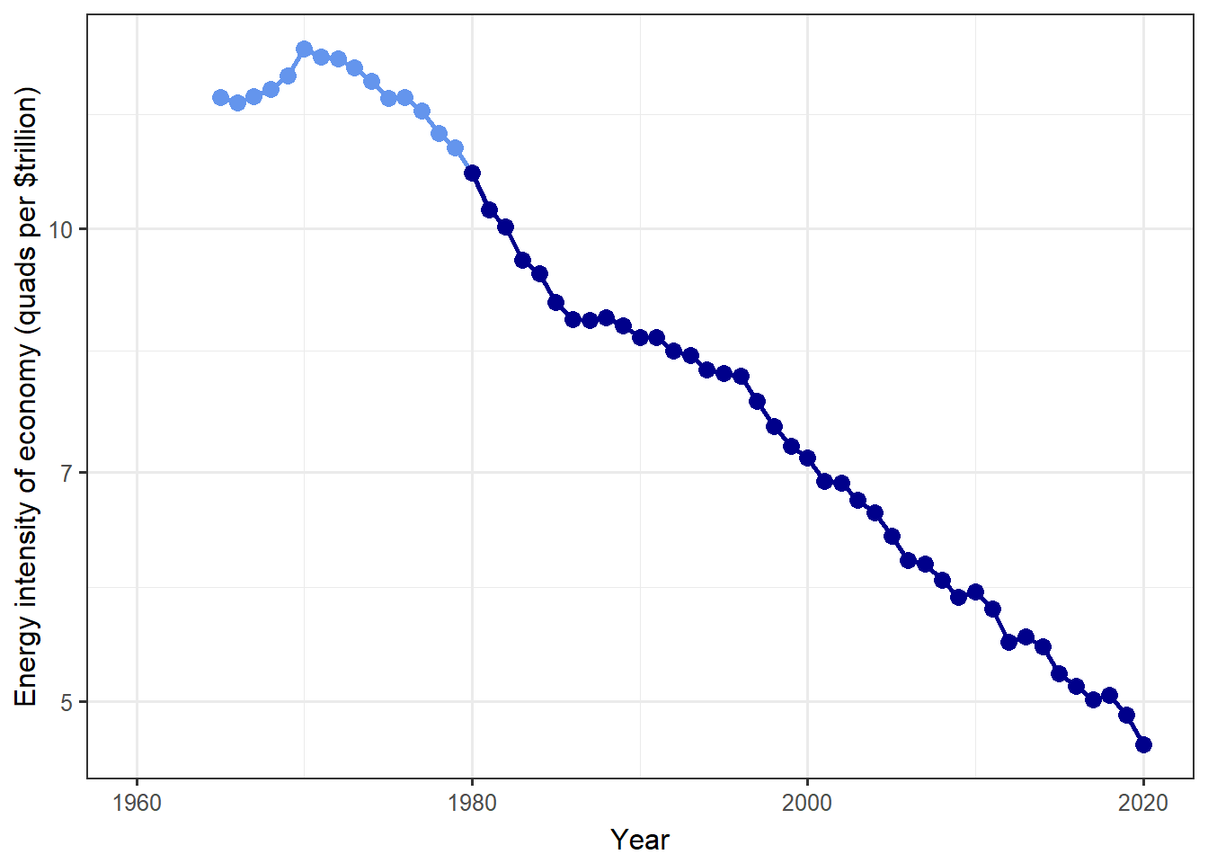

     Use plots like the one above to examine trends in P, g, e, and f. Be sure to set log_scale = TRUE in the plot_kaya function because a constant percentage rate of change corresponds to a linear trend in the logarithm of the variable.

3. In your report, discuss whether you anticipate a problem if we make policy by assuming that the Kaya identity variables will follow the trend line for the next several decades?

4. Next, calculate the rates of change of P, g, e, and f (the Population, per-capita GDP, energy intensity of the economy, and carbon-intensity of the energy supply) from your starting year through 2020, using the lm function in R.

   A constant rate of change is represented by a linear relationship between the natural logarithm of the kaya variable and time: for the variable P (population), we would write this formula in R as log(P)~year.

   Here is an example of calculating the rate of change of e (the energy intensity of the economy) for the United States, using the variable us_data that you calculated above:

   # Load the broom library for organizing lm results
   library(broom)
   
   e_trend = us_data %>% filter(year >= 1980) %>%
     lm(log(e) ~ year, data = .) %>%
     tidy() %>% 
     filter(term == "year") %>% 
     pull(estimate)

   For more detailed explanation of the code above, see the handout “New Tools for Data Analysis.”

   Here, we find that e_trend = -0.0194 (-1.94% per year).

   You can check your results against the interactive web application by looking at the rates of change reported on the “Trends” tab. Be sure to set the start year on the web app to the same values that you used for calculating the slopes in RMarkdown.

   These numbers are the slopes of the trend lines that you looked at in part 2.

5. Using the rates of change that you determined in part 4, use the formulas from the “Growth Rates and Trends” section to compute the values for P, g, e, and f in the year 2050.

   Next, use the growth rates of P, g, e, and f to calculate the growth rate of the total emissions F. Calculate the total CO₂ emissions (F) from the OECD in 2050, assuming that emissions continue to grow at historical rates.

   It may be useful to define functions for frequently used (e.g., see the example growth function in the handout on “New Tools for Data Analysis”)

   Check your work against the bottom-up numbers in the ``Bottom-Up Analysis’’ table on the bottom of the left-hand pane of the web application.

6. Calculate the emissions target: Set the reference year for emissions reduction to 2005, and set the target emissions reduction to 80%.

   Set the target year in the web app to 2050; set the reference year to 2005; set the emissions reduction to 80%.

   How much CO₂ (F) would the OECD emit in 2050 in order to meet your policy goal?

   Let’s work an example using the Middle East:

   F_2005_middle_east = get_kaya_data("Middle East") %>% 
     filter(year == 2005) %>% pull(F)
   F_2005_middle_east

   ## [1] 1394.057

   middle_east_reduction = 0.32
   F_goal_middle_east = F_2005_middle_east * (1 - middle_east_reduction)
   F_goal_middle_east

   ## [1] 947.9588

   Check this result against the interactive web application.

7. Look up what the CO₂ emission is in 2020 and calculate the rate of change in F that would be necessary to achieve your policy target. For the 2050 calculation:

   1. Calculate the ratio of \(F_{2050}/F_{2020}\).
   2. Take the natural logarithm of this ratio (in R, the natural logarithm function is log(); on your calculator it is “LN”).
   3. Divide the logarithm by the number of years (\(2050 - 2020\)). This is the rate of change of F. A positive number means growth and a negative number means a reduction. The percentage rate of change per year is 100 times this number.

   For our Middle East example:

   F_2017_middle_east = get_kaya_data("Middle East") %>% 
     filter(year == 2017) %>% pull(F)
   r_F_middle_east = log(F_goal_middle_east / F_2017_middle_east) / 
     (2050 - 2017)
    r_F_middle_east

   ## [1] -0.02472985

   so total emissions for the Middle East would need to drop by -2.47% per year between 2020 and 2050

8. Now calculate the decarbonization rate implied by the policy goal. This is the rate of reduction of ef, the carbon intensity of the economy. \(F = Pgef\), so \(r_F = r_P + r_g + r_e + r_f\). Subtract the projected r_P and r_g (look them up in the ``Bottom up Analysis’’ table) from r_F, which you just calculated in step~7, to get the rate of change of ef. Multiply the rate of change of ef by -1 to get the rate of decarbonization (because negative rate of change is a positive rate of decarbonization and vice-versa). Multiply by 100 to get the percent implied rate of decarbonization.

9. How does the implied rate of decarbonization for the OECD compare to the historical rate of decarbonization (i.e., the trend in ef reported in the “Bottom up Analysis” table)?