Lab #3 Lab #3 Answers
PDF version
Lab #3 Answers
Chapter 4 Exercises
Fill in R code for the exercises
(I have put the comment # TODO in all of the code chunks where you need to
do this)
and then fill in the answers where I have marked Answer:.
Be sure to write explanations of your answer and don’t just put numbers with
no text.
Exercise 4.1: Methane
Methane has a current concentration of 1.7 ppm in the atmosphere and is doubling at a faster rate than CO2.
Would an additional 10 ppm of methane in the atmosphere have a larger or smaller impact on the outgoing IR flux than an additional 10 ppm of CO2 at current concentrations?
Hint: See the suggestion in the
lab-03-instructionsdocument.
base_co2 = 400 # parts per million
base_ch4 = 1.7 # parts per million
modtran_baseline = run_modtran(file.path(data_dir,
                                         "ex_4_1_baseline.txt"),
                               co2_ppm = base_co2,
                               ch4_ppm = base_ch4)
modtran_plus_10_co2 = run_modtran(file.path(data_dir,
                                            "ex_4_1_plus_10_co2.txt"),
                                  co2_ppm = base_co2 + 10,
                                  ch4_ppm = base_ch4)
modtran_plus_10_ch4 = run_modtran(file.path(data_dir,
                                            "ex_4_1_plus_10_ch4.txt"),
                                  co2_ppm = base_co2,
                                  ch4_ppm = base_ch4 + 10)
i_out_baseline = modtran_baseline$i_out
i_out_co2 = modtran_plus_10_co2$i_out
i_out_ch4 = modtran_plus_10_ch4$i_out
delta_i_co2 = i_out_co2 - i_out_baseline
delta_i_ch4 = i_out_ch4 - i_out_baseline
Answer: I ran MODTRAN three times. One run was a baseline, which used the current concentrations of CO2 and CH4. Then I ran MODTRAN with the CO2 concentration increased by 10 ppm and I ran it a third time with the baseline value for CO2, but with CH4 increased by 10 ppm.
For the baseline run, the intensity of outgoing longwave light was 298.7. Watts per square meter. Increasing CO2 by 10 ppm decreased the outgoing longwave light by 0.13 W/m2, and increasing CH4 by 10 ppm decreased the outgoing longwave light by 3.11 W/m2, which is around 25. times as much as for CO2.
The difference is because absorption for CO2 is strongly saturated, but the absorption for CH4 is not saturated. Another way to think about this is that a 10 ppm increase in CO2 increases the atmospheric concentration by 2.5% and a 10 ppm increase in CH4 increases the atmospheric concentration by 590.%.
Where in the spectrum does methane absorb? What concentration does it take to begin to saturate the absorption in this band? Explain what you are looking at to judge when the gas is saturated.
Hints:
See the hints in thelab-03-instructionsdocument.
ch4_values = c(0, 2^seq(0,7))
sat_data = tibble()
for (ch4 in ch4_values) {
   filename = file.path(data_dir, str_c("ex_4_1_ch4_", ch4, ".txt"))
   if (file.exists(filename)) {
      mod_data = read_modtran(filename)
   } else {
      mod_data = run_modtran(filename, co2_ppm = 0, ch4_ppm = ch4,
                             trop_o3_ppb = 0, strat_o3_scale = 0,
                             h2o_scale = 0, freon_scale = 0,
                             atmosphere = "standard", altitude_km = 70)
   }
   p = plot_modtran(mod_data, descr = str_c(ch4, " ppm methane"))
   plot(p)
}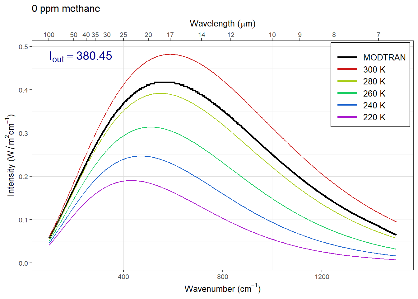
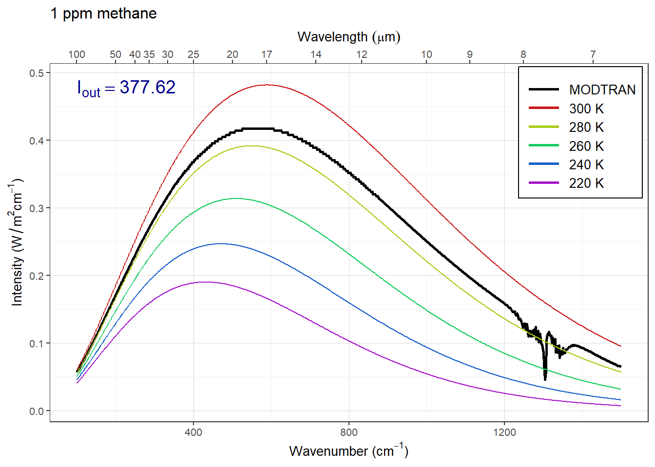
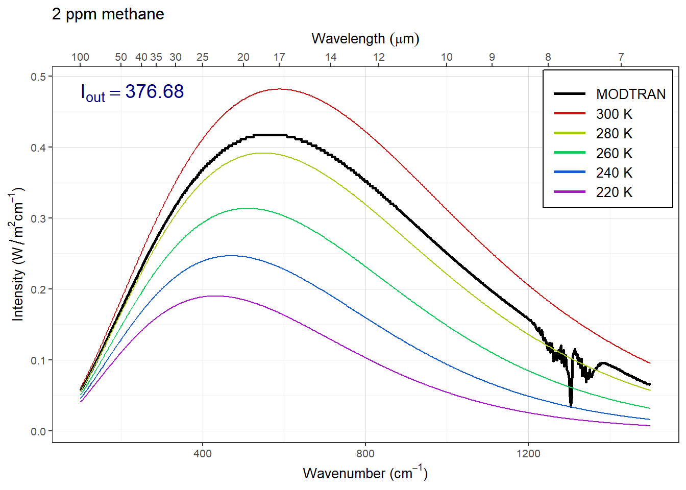


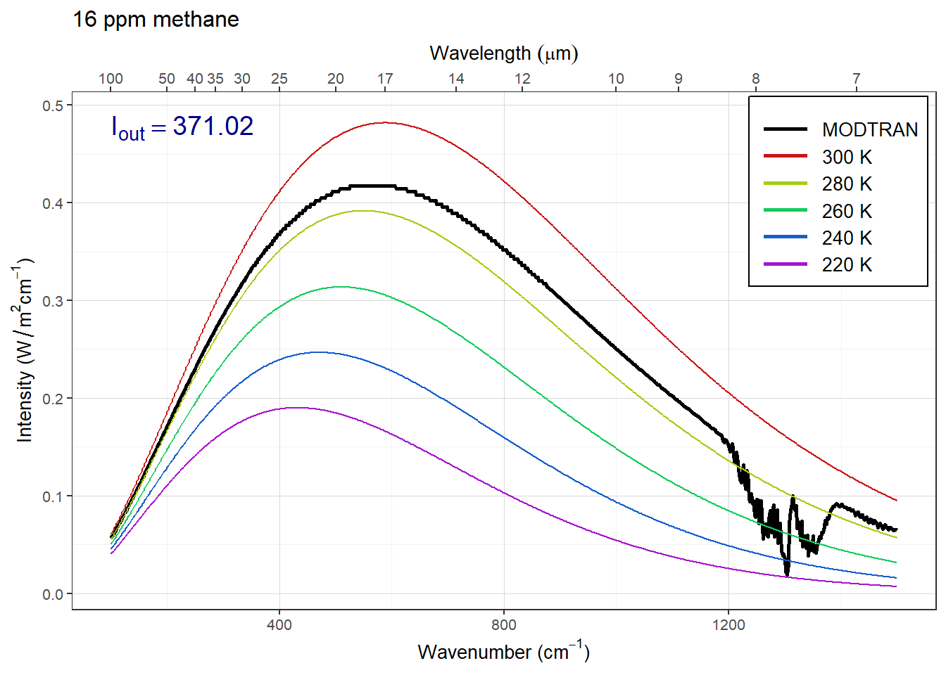
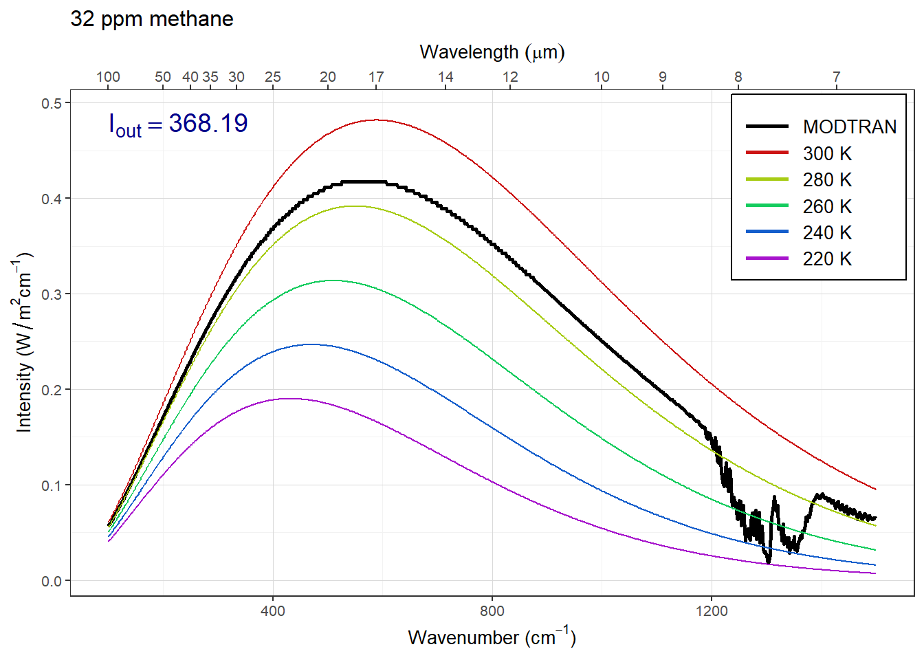
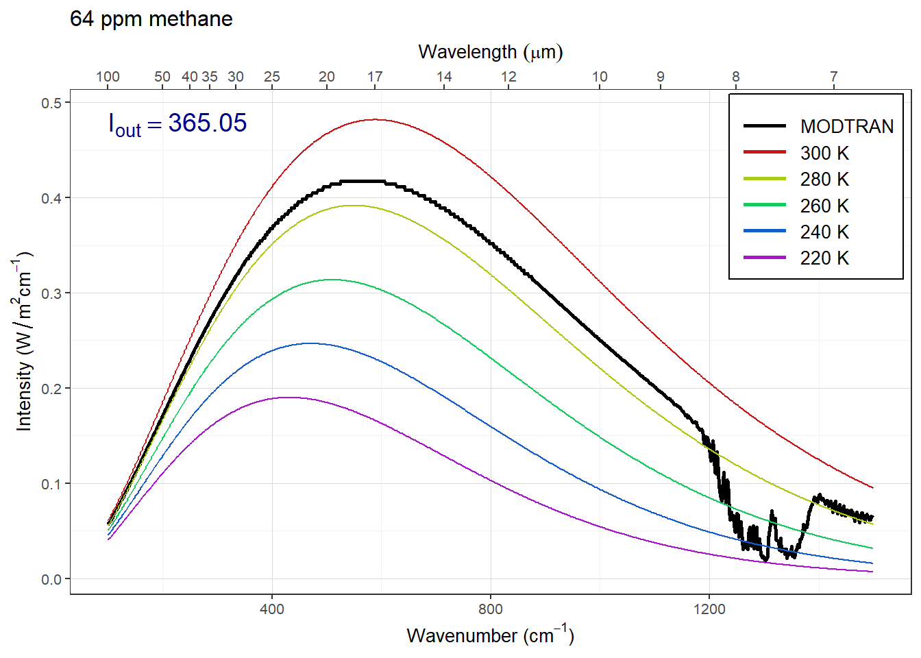

Answer: The plots above show the MODTRAN spectrum with all gases set to zero except methane. Methane absorbs most strongly around 1300 wavenumbers.
As we increase the methane concentration, the big spike around 1300 wavenumbers gets bigger until it bottoms out on the black line. This happens somwhere around 8, 16, or 32 ppm, so any of those anwers would be correct. But the spectrum is complicated and so is its saturation, so other answers are plausible if they are supported by sound reasoning.
Would a doubling of methane have as great an impact on the heat balance as a doubling of CO2?
Hint: See the suggestion in the
lab-03-instructionsdocument.
base_co2_ppm = 400
base_methane_ppm = 1.7
baseline =   read_modtran(file.path(data_dir, "ex_4_1_baseline.txt"))
double_co2 = run_modtran(file.path(data_dir, "ex_4_1_2x_co2.txt"),
                         co2_ppm = 2 * base_co2_ppm,
                         ch4_ppm = base_methane_ppm)
double_ch4 = run_modtran(file.path(data_dir, "ex_4_1_2x_ch4.txt"),
                         co2_ppm = base_co2_ppm,
                         ch4_ppm = 2 * base_methane_ppm)
i_out_baseline = baseline$i_out
i_out_co2 = double_co2$i_out
i_out_ch4 = double_ch4$i_out

delta_i_out_co2 = i_out_co2 - i_out_baseline
delta_i_out_ch4 = i_out_ch4 - i_out_baseline
Answer: The baseline value for Iout is 298.7 W/m2. If we double CO2, it drops to 295.3 W/m2, a decrease of -3.3 W/m2, and if we double CH4, it drops to 297.8 W/m2, a decrease of -0.88 W/m2. Doubling CO2 has the larger effect because there is a lot more CO2 in the atmosphere and that is more important than how saturated its absorption is.
You can see this if you look at the plots below. Notice that the effect of doubling CO2 isn’t to make the big CO2 absorption feature get deeper, but to make it wider. You can see this if you compare the baseline to the doubled CO2 spectrum where the purple spectrum crosses the yellow blackbody curve near 600 wavenumbers and around 750 wavenumbers. Compare this to the very small change in the methane spike near 1300 wavenumbers (you have to look very carefully at the doubled methane spectrum to notice this).
plot_modtran(baseline, descr = "Baseline spectrum")
plot_modtran(double_co2, descr = "Doubled CO2")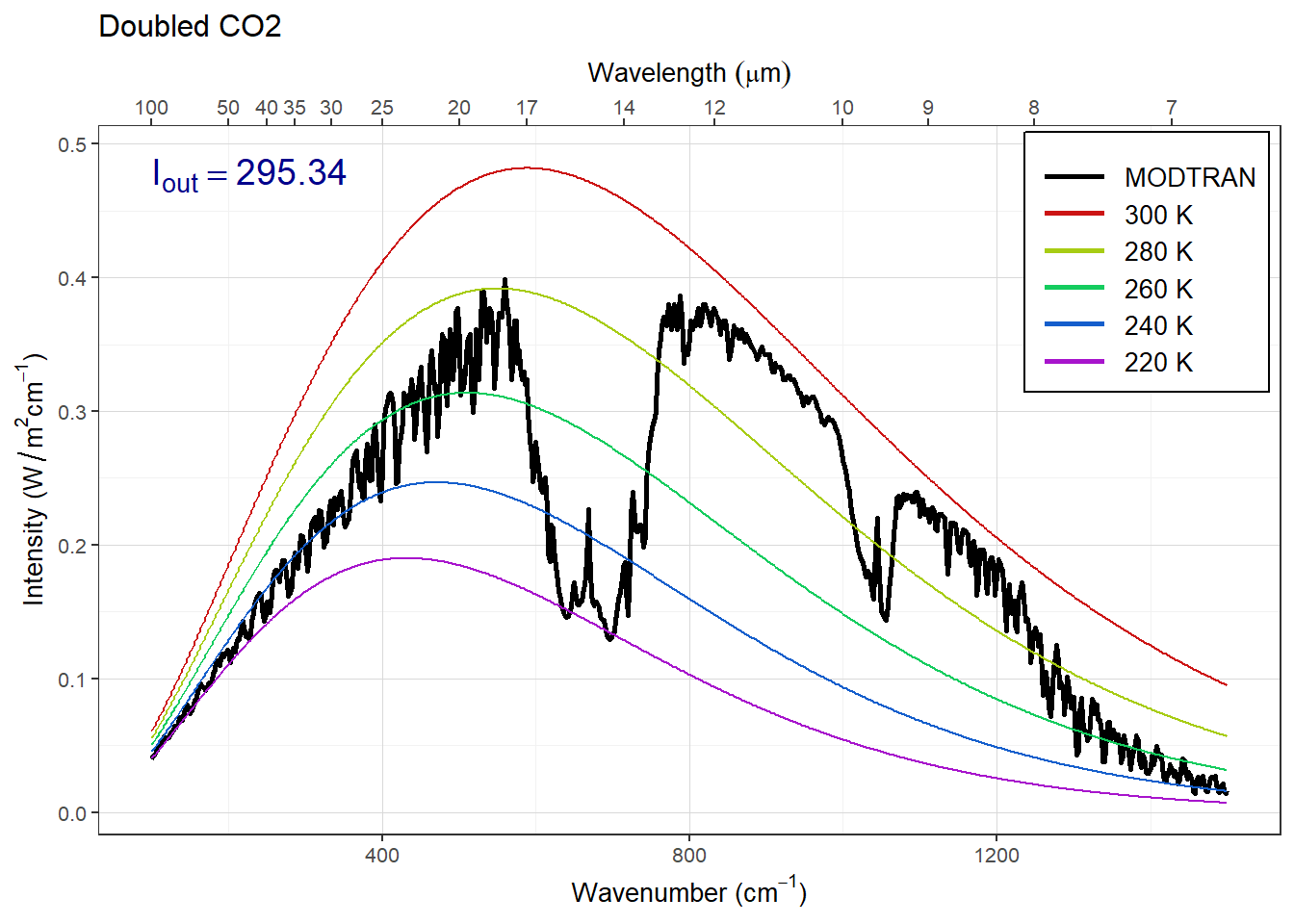
plot_modtran(double_ch4, descr = "Doubled CH4")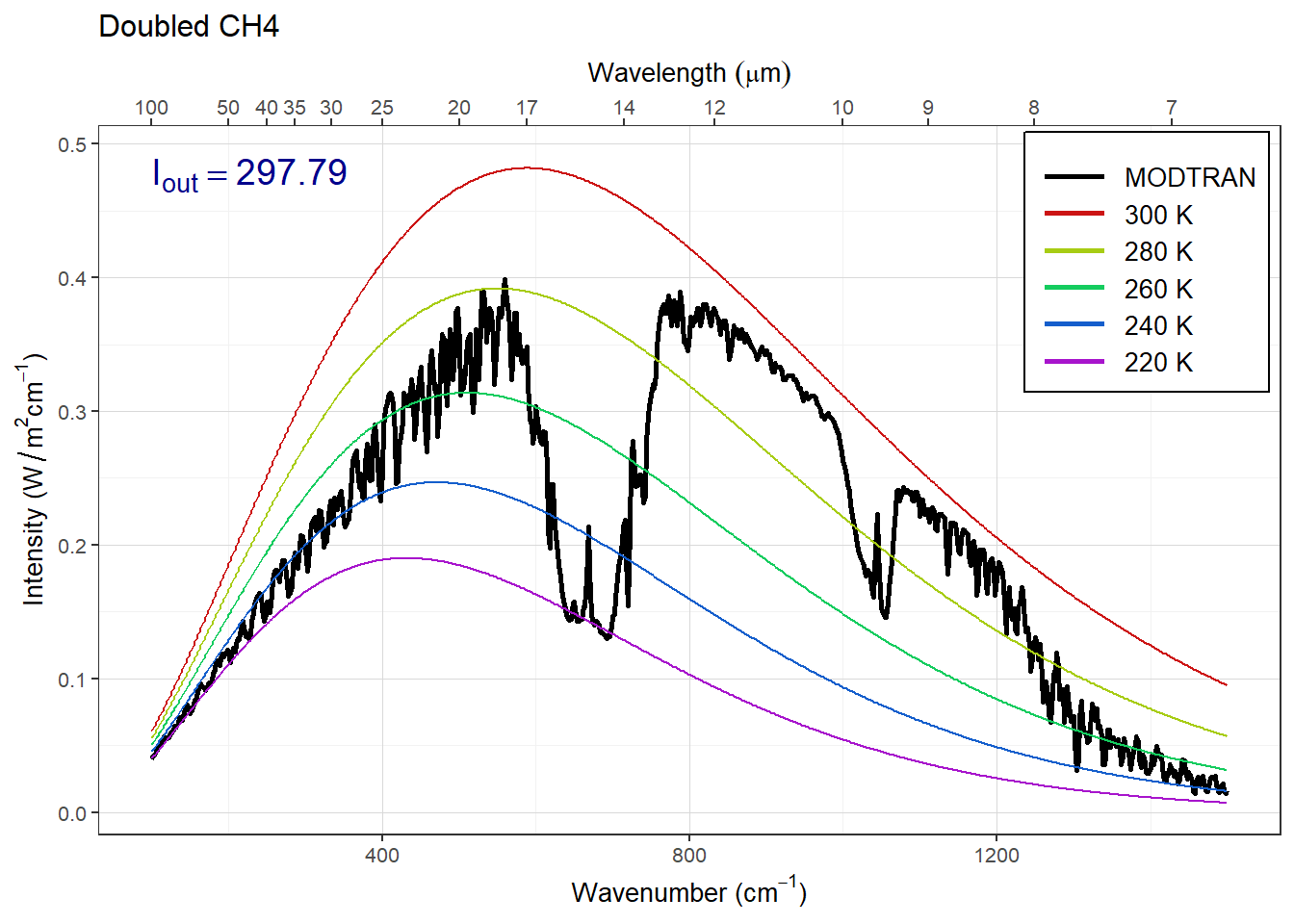
- What is the “equivalent CO2” of doubling atmospheric methane? That is to say, how many ppm of CO2 would lead to the same change in outgoing IR radiation energy flux as doubling methane? What is the ratio of ppm CO2 change to ppm methane change?
matching_methane = 13
modtran_match_ch4 = run_modtran(file.path(data_dir, "ex_4_1_ch4_match.txt"),
                                co2_ppm = 400, ch4_ppm = matching_methane)
Answer:
When we double CO2, Iout is
rformat_md(i_out_co2, digits = 4)`W/m2.
We need to adjust CH4 to produce the same Iout with the defailt value of
400 ppm CO2. After some trial and error, this turns out to be about
13 ppm,
which has Iout = 295.34
Exercise 4.2: CO2 (Graduate students only)
Is the direct effect of increasing CO2 on the energy output at the top of the atmosphere larger in high latitudes or in the tropics?
Hint: See the hint in the
lab-03-instructionsdocument.
modtran_lat_df = tibble()
for (atmos in c("tropical", "midlatitude summer", "subarctic summer"
                #, "midlatitude winter", "subarctic winter"
)) {
  for (co2 in c(400, 800)) {
    filename = file.path(data_dir,
                         str_c("ex_4_2_", atmos, "_co2_", co2, ".txt"))
    if (file.exists(filename)) {
      mod_data = read_modtran(filename)
    } else {
      mod_data = run_modtran(filename, atmosphere = atmos, co2_ppm = co2)
    }
    modtran_lat_df = bind_rows(modtran_lat_df,
                               tibble(co2 = co2, atmos = atmos,
                                      i_out = mod_data$i_out))
  }
}

modtran_lat_df = modtran_lat_df %>%
  mutate(co2 = str_c("co2_", co2)) %>%
  pivot_wider(names_from = "co2", values_from = "i_out") %>%
  mutate(delta_i = co2_400 - co2_800) %>%
  arrange(desc(delta_i))
kable(modtran_lat_df, digits = 1)| atmos | co2_400 | co2_800 | delta_i |
|---|---|---|---|
| tropical | 298.7 | 295.3 | 3.3 |
| midlatitude summer | 289.7 | 286.7 | 3.0 |
| subarctic summer | 270.9 | 268.4 | 2.5 |
Answer: When atmospheric CO2 doubles, the greatest change in Iout occurs in the tropics, followed by the midlatitudes, and the smallest change occurs at high latitudes in the subarctic.
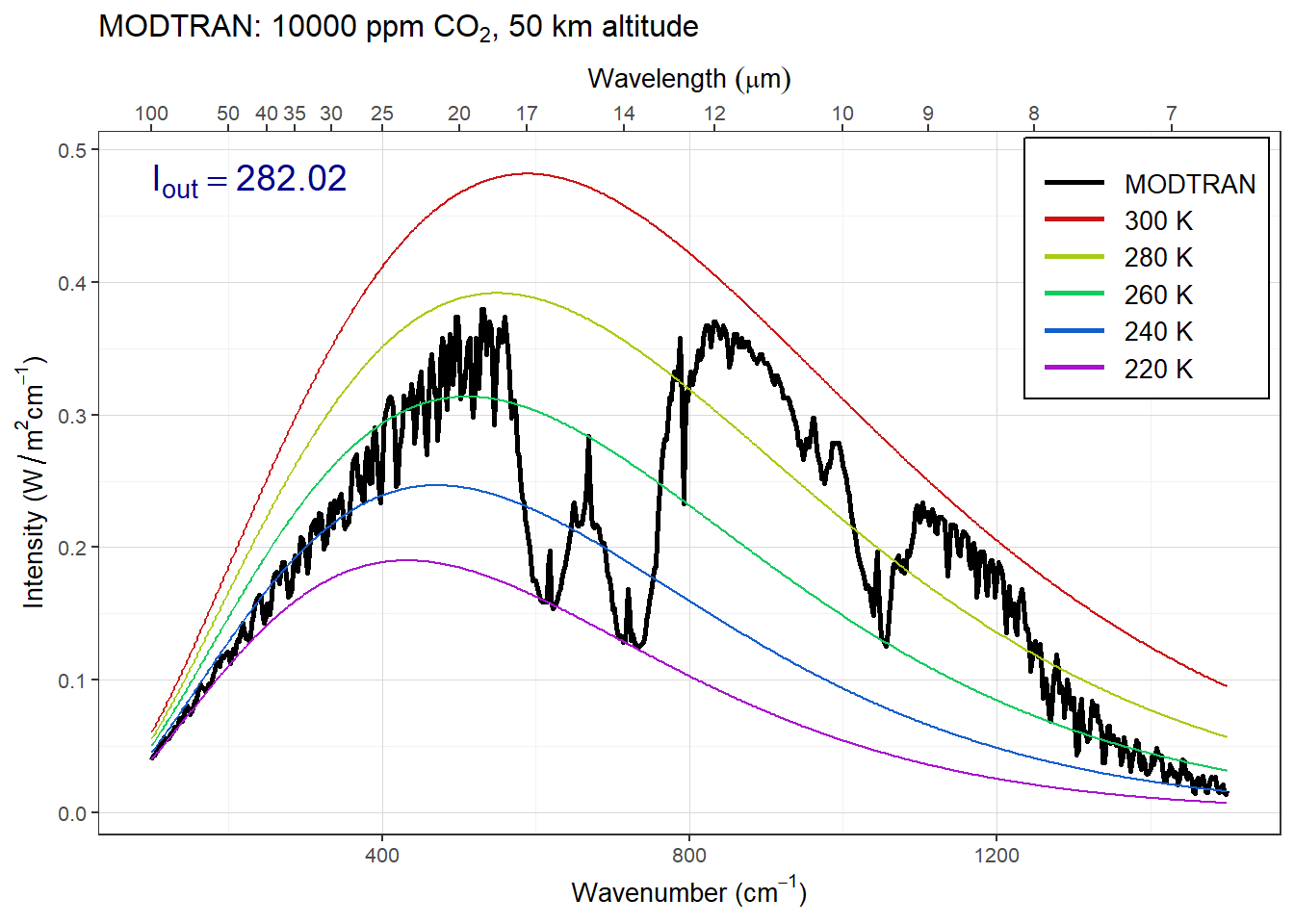
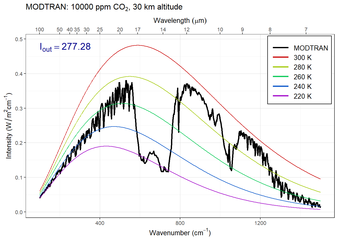
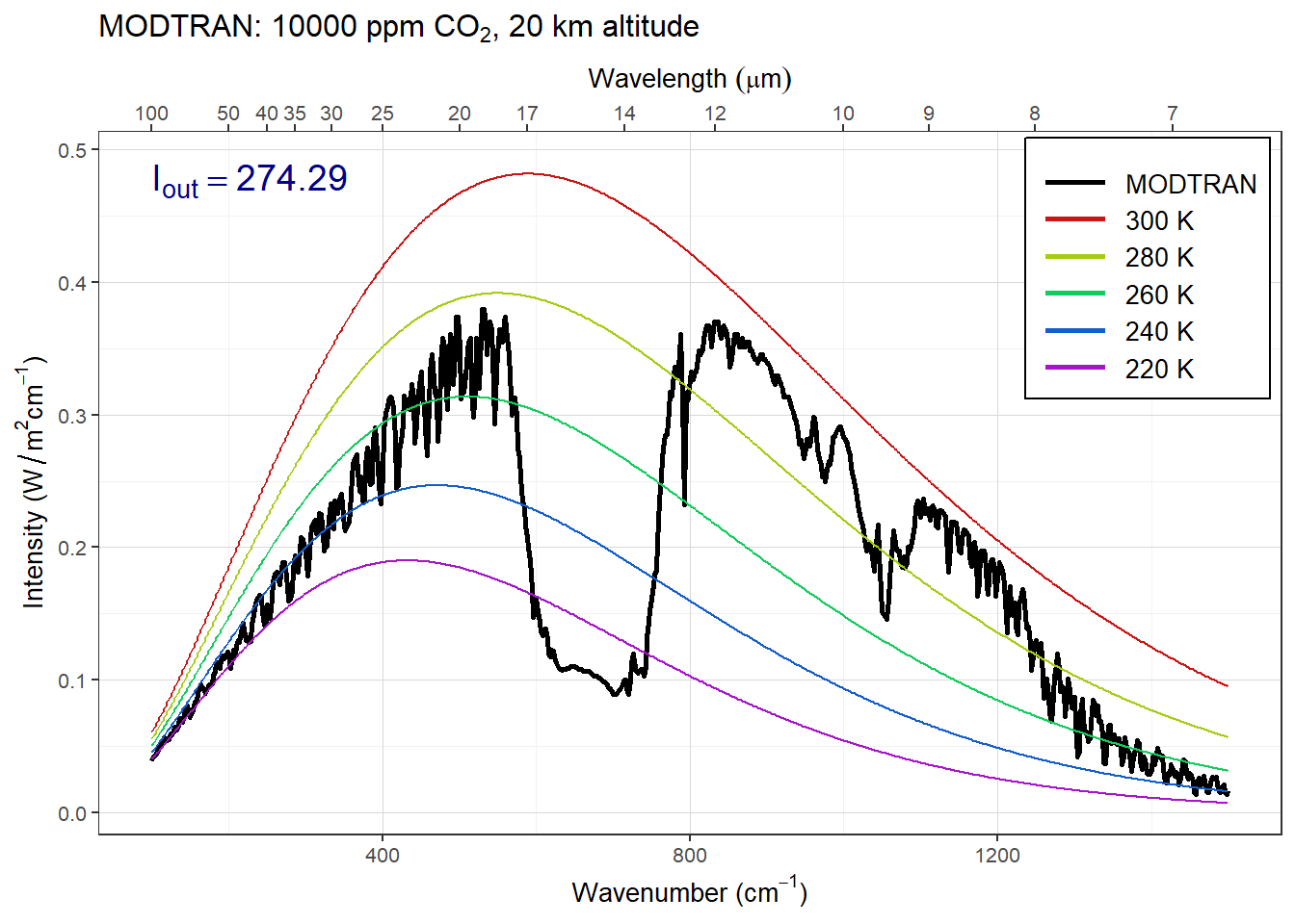
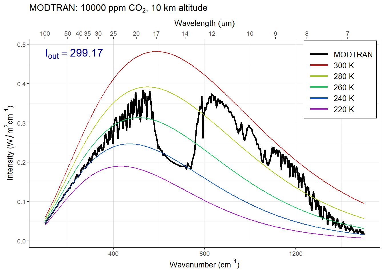
Set pCO2 to an absurdly high value of 10,000 ppm. You will see a spike in the CO2 absorption band. What temperature is this light coming from? Where in the atmosphere do you think this comes from?
Now turn on clouds and run the model again. Explain what you see. Why are night-time temperatures warmer when there are clouds?
Hint: See the hint in the
lab-03-instructionsdocument and for the second part of this exercise, try using “altostratus” clouds.
The figure below shows the spectrum with a high concentration of CO2.
high_co2 = 1E4
for (z in c(70, 60, 50, 40, 30, 20, 10)) {
  filename = file.path(data_dir, str_c("ex_4_2_alt_", z, ".txt"))
  if (file.exists(filename)) {
    modtran_high_co2 = read_modtran(filename)
  } else {
    modtran_high_co2 = run_modtran(filename, co2_ppm = high_co2,
                                   altitude_km = z)
  }
  p = plot_modtran(modtran_high_co2)
  plot(p)
}


high_co2 = 1E4
modtran_high_co2 = run_modtran(file.path(data_dir,
                                         "ex_4_2_hi_co2_clear.txt"),
                               co2_ppm = high_co2)
plot_modtran(modtran_high_co2)![]()
high_co2 = 1E4
modtran_high_co2 = run_modtran(file.path(data_dir,
                                         "ex_4_2_hi_co2_cloudy.txt"),
                               co2_ppm = high_co2, clouds = "altostratus")
plot_modtran(modtran_high_co2)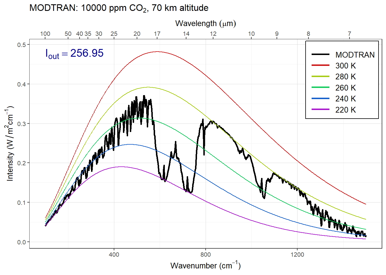
Answer: The spike in the CO2 absorption feature gets smaller as the sensor altitude drops below about 40 km, and disappears entirely as the sensor drops below 30 km. This means that the spike must be coming from the region of the atmosphere between 30 and 40 km.
When you add altostratus clouds to the atmosphere there isn’t much change in the emission from the big absorption spikes but the emission from the window region of the spectrum drops considerably. The clouds block longwave emissions in the window region. This traps heat near the surface and is one reason why cloudy nights tend to be warmer than clear nights.
Exercise 4.3: Water vapor
Our theory of climate presumes that an increase in the temperature at ground level will lead to an increase in the outgoing IR energy flux at the top of the atmosphere.
How much extra outgoing IR would you get by raising the temperature of the ground by 5°C? What effect does the ground temperature have on the shape of the outgoing IR spectrum and why?
Hint: See the hint in the
lab-03-instructionsdocument.
modtran_baseline = run_modtran(file.path(data_dir, "ex_4_3_baseline.txt"))
modtran_plus_5 = run_modtran(file.path(data_dir, "ex_4_3_t_plus_5"),
                             delta_t = 5)

p_baseline = plot_modtran(modtran_baseline, descr = "Baseline spectrum")
p_plus_5 = plot_modtran(modtran_plus_5,
                        descr = "Ground temperature raised 5K")
plot(p_baseline)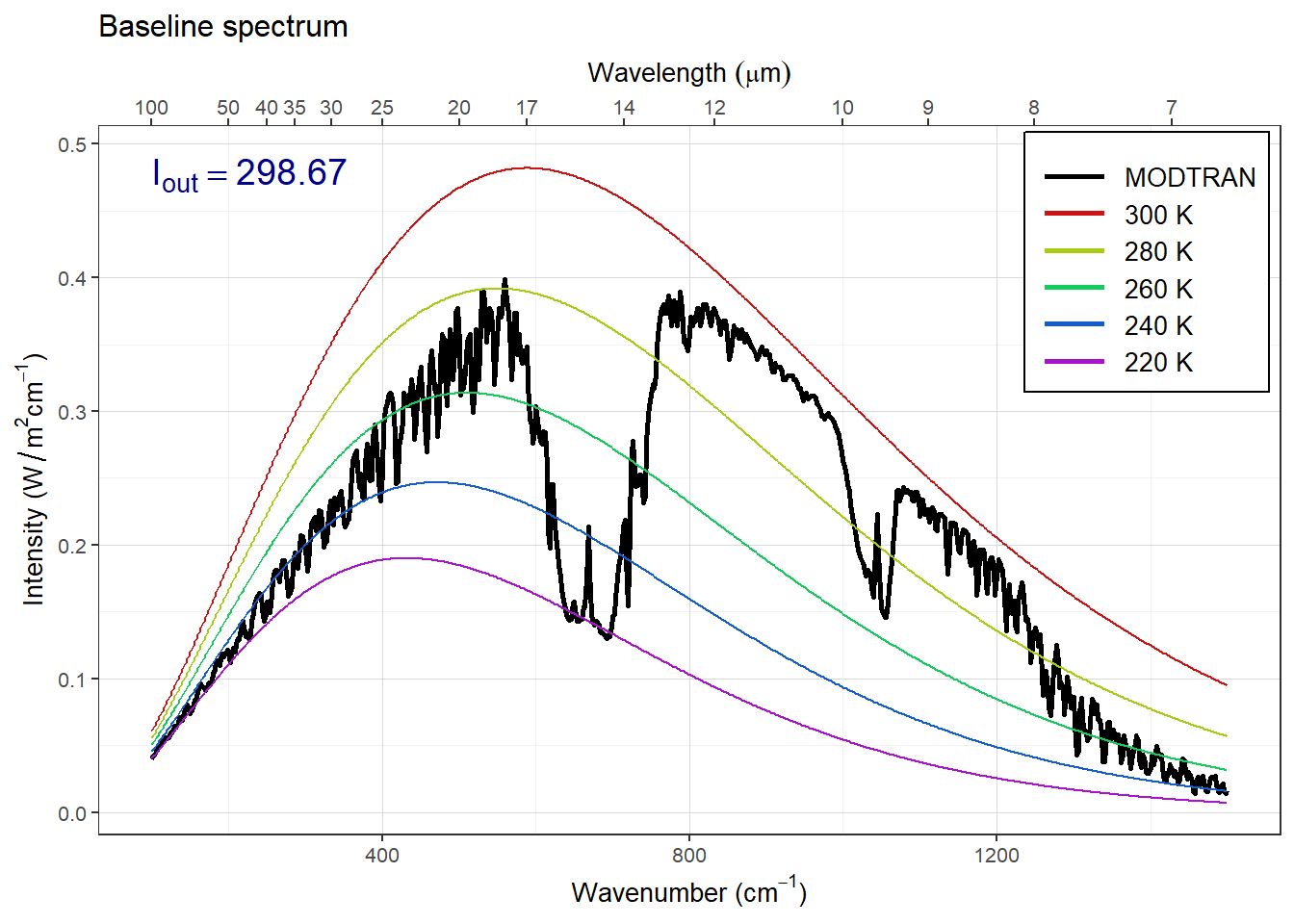
plot(p_plus_5)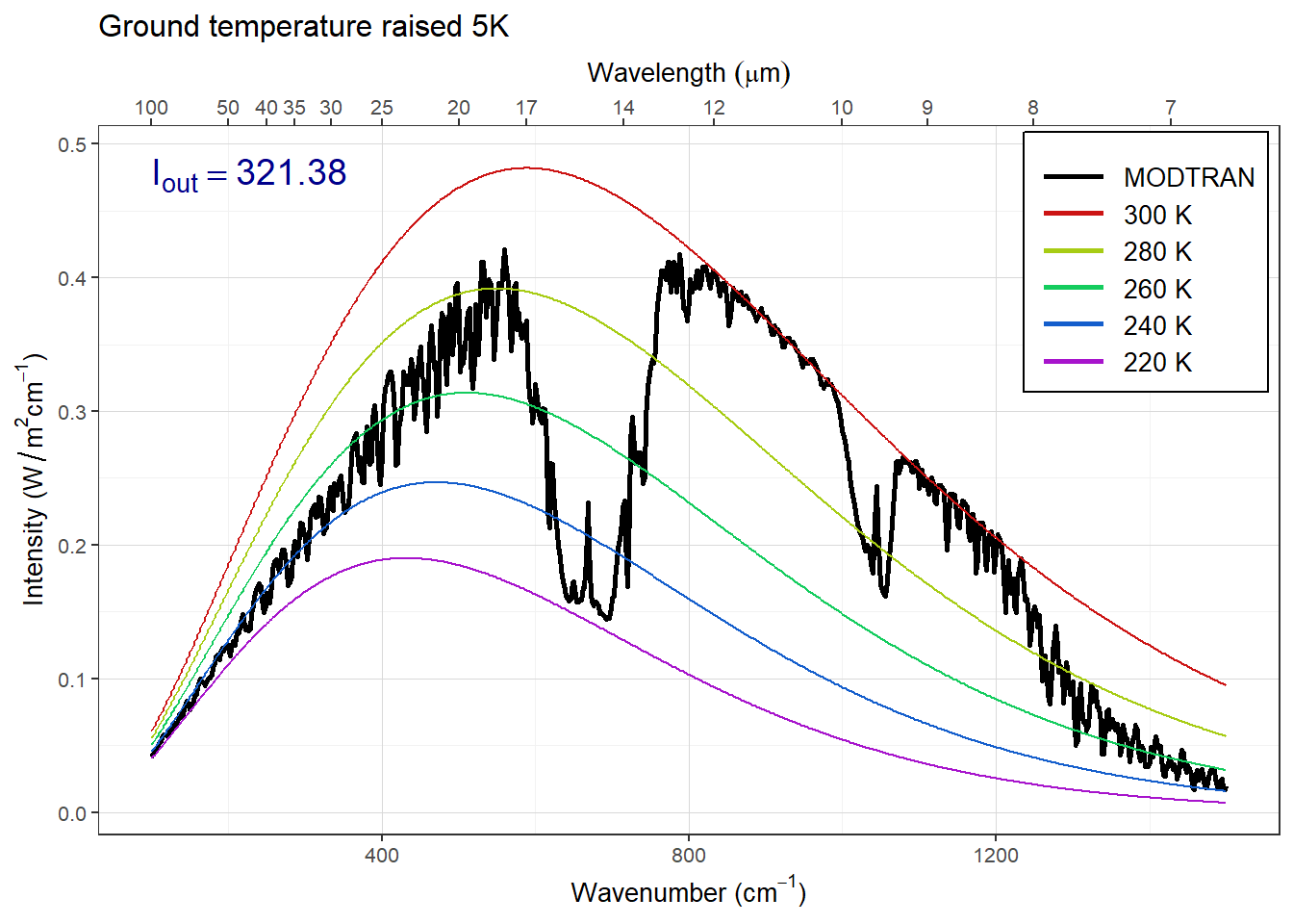
Answer: Raising the ground temperature raises the entire spectrum.
More water can evaporate into warm air than into cool air. Change the model settings to hold the water vapor at constant relative humidity rather than constant vapor pressure (the default), calculate the change in outgoing IR energy flux for a 5°C temperature increase. Is it higher or lower? Does water vapor make the Earth more sensitive to CO2 increases or less sensitive?
Note: By default, the MODTRAM model holds water vapor pressure constant, but you can set it to hold relative humidity constant instead with the option
h2o_fixed = "relative humidity", like this:run_modtran(file_name, delta_t = 5, h2o_fixed = "relative humidity").
modtran_vp = run_modtran(file.path(data_dir, "ex_4_3_vap_press.txt"),
                         delta_t = 5, h2o_fixed = "vapor pressure")
modtran_rh = run_modtran(file.path(data_dir, "ex_4_3_rel_humid.txt"),
                         delta_t = 5, h2o_fixed = "relative humidity")

i_out_baseline = modtran_baseline$i_out
i_out_vp = modtran_vp$i_out
i_out_rh = modtran_rh$i_out

p_vp = plot_modtran(modtran_vp, descr = "Constant vapor pressure",
                    i_out_ref = i_out_baseline)
p_rh = plot_modtran(modtran_rh, descr = "Constant relative humidity",
                    i_out_ref = i_out_baseline)
plot(p_vp)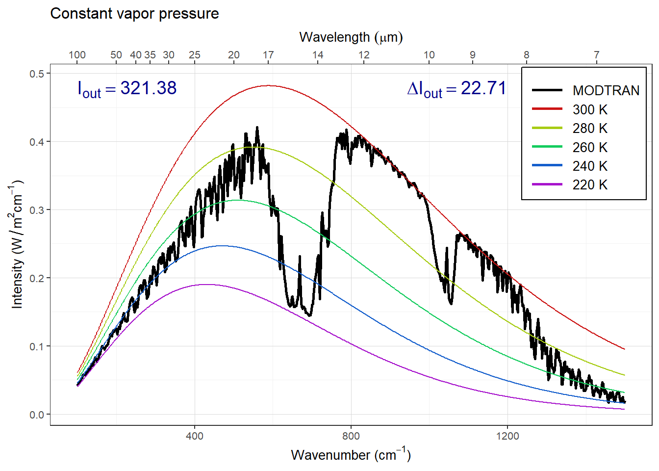
plot(p_rh)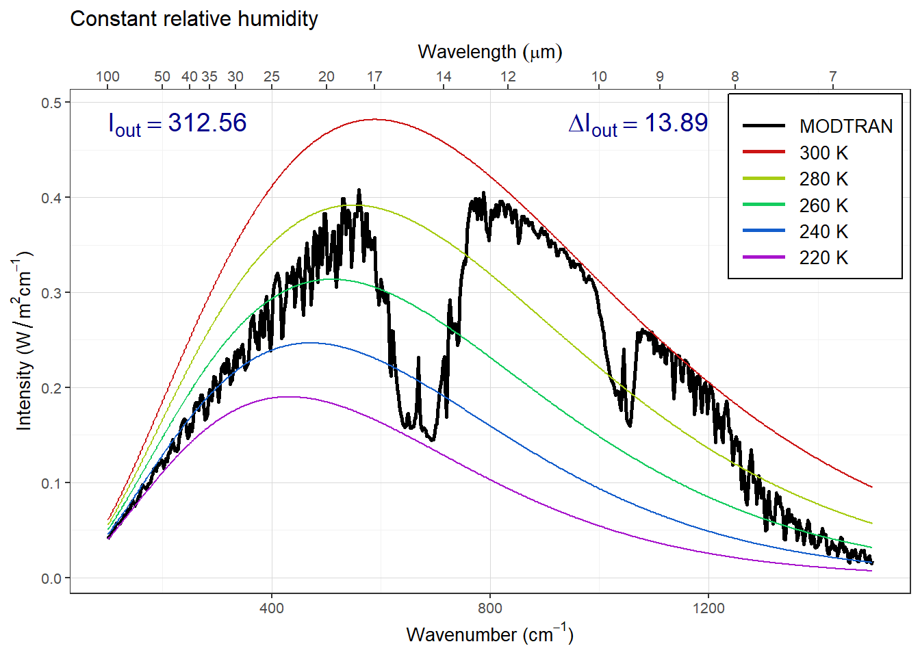
Answer: Raising the surface temperature has a bigger effect on Iout when water vapor pressure is fixed than when relative humidity is fixed. This means that compensating for a change in CO2 would require a bigger change in temperature with fixed relative humidity, so the climate is more sensitive to changes in CO2 when relative humidity is fixed.
Now see this effect in another way.
Starting from the default base case, record the total outgoing IR flux.
Now double CO2. The temperature in the model stays the same (that’s how the model is written), but the outgoing IR flux goes down.
Using constant water vapor pressure, adjust the temperature offset until you get the original IR flux back again. Record the change in temperature.
Now repeat the exercise, but holding the relative humidity fixed instead of the water vapor pressure.
The ratio of the warming when you hold relative humidity fixed to the warming when you hold water vapor pressure fixed is the feedback factor for water vapor. What is it?
modtran_baseline = read_modtran(file.path(data_dir, "ex_4_3_baseline.txt"))
i_baseline = modtran_baseline$i_out

modtran_2xco2 = run_modtran(file.path(data_dir, "ex_4_3_2x_co2_vp.txt"),
                                      co2_ppm = 800)
i_2x_vp = modtran_2xco2$i_out

dt_vp = 0.76
modtran_vp_dt = run_modtran(file.path(data_dir, "ex_4_3_vp_dt.txt"),
                            co2_ppm = 800, delta_t = dt_vp)
i_vp_dt = modtran_vp_dt$i_out

modtran_2x_rh = run_modtran(file.path(data_dir, "ex_4_3_2x_co2_rh_.txt"),
                            co2_ppm = 800, h2o_fixed = "relative humidity")
i_2x_rh = modtran_2x_rh$i_out

dt_rh = 1.21
modtran_rh_dt = run_modtran(file.path(data_dir, "ex_4_3_rh_dt.txt"),
                            co2_ppm = 800, delta_t = dt_rh,
                            h2o_fixed = "relative humidity")
i_rh_dt = modtran_rh_dt$i_out

feedback_factor = dt_rh / dt_vp
Answer: In the baseline case, Iout = 298.67 W/m2. When we double CO2 with constant water vapor pressure, Iout drops to 295.34 W/m2 and we have to raise the ground temperature by 0.760 K to bring Iout back to Iout = 298.67 W/m2.
When we double CO2 with constant water relative humidity, Iout drops to 295.34 W/m2 and we have to raise the ground temperature by 1.21 K to bring Iout back to Iout = 298.67 W/m2.
The feedback factor is the ratio of the temperature change with relative humidity fixes to the temperature change with vapor pressure fixed: f = 1.59.
Notice that there is no difference between holding vapor pressure constant and holding relative humidity constant until the temperature changes.
Chapter 5 Exercise
Exercise 5.2: Skin Height
Run the MODTRAN model using the “tropical” atmosphere, without clouds, and with the present-day CO2 concentration (400 ppm). Use the ground temperature reported by the model to calculate \(\varepsilon \sigma T_{\text{ground}}^4\), the heat flux emitted by the ground. Assume \(\varepsilon = 1\), and I have already provided the value of the Stefan-Boltzmann constant \(\sigma\), as the R variable
sigma_sb, which equals 5.670×10⁻⁸. (I defined it in the script “utils.R”, which I loaded in the “setup” chunk in the RMarkdown document).Next, look at the outgoing heat flux at the top of the atmosphere (70 km) (Iout) reported by the MODTRAN model. Is it greater or less than the heat flux that you calculated was emitted by the ground?
baseline = run_modtran(file.path(data_dir, "ex_5_2_baseline.txt"),
                       co2_ppm = 400, atmosphere = "tropical",
                       clouds = "none")
epsilon = 1.0
t_ground = baseline$t_ground
i_ground = epsilon * sigma_sb * t_ground^4
i_atmos_up = baseline$i_out
Answer: Tground = 299.7 K, so \(I_{\text{out}} = \varepsilon \sigma T_{\text{ground}}^4 = 457.5\) W/m2. The MODTRAN model reports Iout = 298.7 W/m2. Iground is roughly 1.5 times greater than Iout.
Use the outgoing heat flux at the top of the atmosphere (Iout) to calcuate the skin temperature (use the equation \(I_{\text{out}} = \varepsilon \sigma T_{\text{skin}}^4)\)). What is the skin temperature, and how does it compare to the ground temperature and the temperature at the tropopause, as reported by the MODTRAN model (
t_tropo)?Assuming an environmental lapse rate of 6K/km, and using the skin temperature that you calculated above, and the ground temperature from the model, what altitude would you expect the skin height to be?
lapse_rate = 6.0 # Kelvin/km
t_tropo = baseline$t_tropo
t_skin = (i_atmos_up / (epsilon * sigma_sb))^0.25
h_skin = (t_ground - t_skin) / lapse_rate
Answer: The skin temperature is given by
\[T_{\text{skin}} = \sqrt[4]{\frac{I_{\text{out}}}{\varepsilon \sigma}}\] Tskin = 269.4 K, which is 30.3 K less than the ground temperature and greater than the tropopause temperature Ttropo = 194.8. The skin height is \[h_{\text{skin}} = \frac{T_{\text{ground}} - T_{\text{skin}}}{\text{lapse rate}}\] so with a lapse rate of 6 K/km, hskin = 5.1 km.
Double the CO2 concentration and run MODTRAN again. Do not adjust the ground temperature. Repeat the calculations from (b) of the skin temperature and the estimated skin height.
What is the new skin temperature? What is the new skin height?
modtran_2x_co2 = run_modtran(file.path(data_dir, "ex_5_2_2x_co2_clear.txt"),
                             co2_ppm = 800, atmosphere = "tropical",
                             clouds = "none")
i_out_2x = modtran_2x_co2$i_out
t_skin_2x = (i_out_2x / (epsilon * sigma_sb))^0.25
h_skin_2x = (t_ground - t_skin_2x) / lapse_rate
Answer: The new Iout is 295.3 W/m2, so the new Tskin is 268.6 K, which implies that the new skin height is 5.2 km, 0.13 km higher than for today’s CO2 concentration.
Put the CO2 back to today’s value, but add cirrus clouds, using the “standard cirrus” value for the clouds. Repeat the calculations from (b) of the skin temperature and the skin height.
What is the new skin temperature? What is the new skin height? Did the clouds or the doubled CO2 have a greater effect on the skin height?
modtran_cirrus = run_modtran(file.path(data_dir, "ex_5_2_cirrus.txt"),
                             co2_ppm = 400, atmosphere = "tropical",
                             clouds = "standard cirrus")
i_out_cirrus = modtran_cirrus$i_out
t_skin_cirrus = (i_out_cirrus / (epsilon * sigma_sb))^0.25
h_skin_cirrus = (t_ground - t_skin_cirrus) / lapse_rate
Answer: The new skin height is 5.9 km, which is 0.68 km higher than for the doubled CO2. To put this in context, doubling CO2 raises the skin hight by 0.13 km and adding cirrus clouds raises the skin height by 0.81, so the cirrus clouds have a much bigger effect on the climate.
