Lab #4 Lab #4 Answers
PDF version
Lab #4 Answers
General Instructions
In the past three weeks, we focused on mastering many of the basics of using R and RMarkdown. For this week’s lab, when you write up the answers, I would like you to think about integrating your R code chunks with your text.
For instance, you can describe what you’re going to do to answer the question, and then for each step, after you describe what you’re going to do in that step, you can include an R code chunk to do what you just described, and then the subsequent text can either discuss the results of what you just did or describe what the next step of the analysis will do.
This way, your answer can have several small chunks of R code that build on each other and follow the flow of your text.
For this lab, you will use the RRTM model, which includes both radiation and convection.
Exercise 1: Lapse Rate
Run the RRTM model in its default configuration and then vary the lapse rate
from 0 to 10 K/km. For each value of the lapse rate, adjust the surface
temperature until the earth loses as much heat as it gains (i.e., the value of
Q in the run_rrtm model output is zero.)
It will probably be easier to do this with the interactive version of the RRTM
model at http://climatemodels.uchicago.edu/rrtm/ than with the R interface
run_rrtm.
Make a tibble containing the values of the lapse rate and the corresponding equilibrium surface temperature, and make a plot with lapse rate on the horizontal axis and surface temperature on the vertical axis.
Describe how the equilibrium surface temperature varies as the lapse rate varies.
Exercise 1 Report:
I varied the lapse rate from 0 to 10 Kelvin/km in steps of 1 K/km. At each value of the lapse rate, I manually adjusted the surface temperature in the interactive RRTM model until the heat budget was balanced (the model reported that “If the Earth has these properties … then it loses as much energy as it gains.”).
lapse_vs_t = tibble( lapse = seq(0, 10),
                     t_surf = c(256.05, 264.66, 271.65, 276.95, 280.75, 283.15,
                                284.40, 285.00, 285.25, 285.30, 285.30))
kable(lapse_vs_t, col.names = c("Lapse rate", "Surface temperature"))| Lapse rate | Surface temperature |
|---|---|
| 0 | 256.05 |
| 1 | 264.66 |
| 2 | 271.65 |
| 3 | 276.95 |
| 4 | 280.75 |
| 5 | 283.15 |
| 6 | 284.40 |
| 7 | 285.00 |
| 8 | 285.25 |
| 9 | 285.30 |
| 10 | 285.30 |
The figure below shows the results. As the lapse rate increases, the change in surface temperature becomes smaller and smaller. At the last step, from 9 to 10 K/km, the surface temperature did not change at all.
ggplot(lapse_vs_t, aes(x = lapse, y = t_surf)) +
   geom_line(size = 1, color = "darkblue") +
   geom_point(size = 3, color = "darkblue") +
   labs(x = "Lapse rate (K/km)", y = "Ground temperature (K)")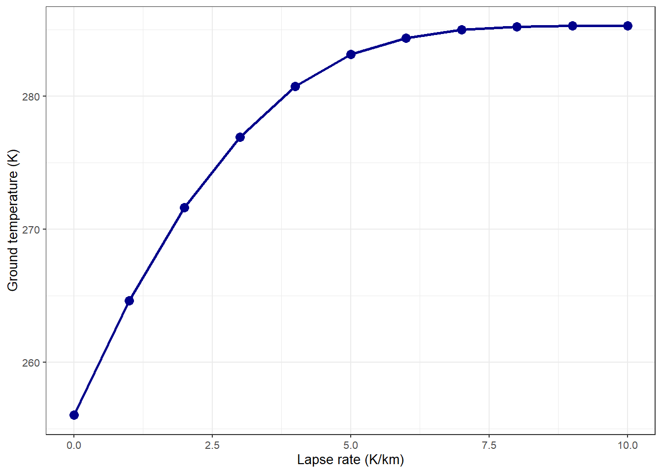
Figure 1: Equilibrium surface temperature versus lapse rate.
Explanation:
Students don’t need to have this detail in their reports, but the reason this is happening is that the closer the basic environmental lapse rate gets to the dry adiabatic lapse rate, the less stable the atmosphere is and the easier it is for solar heating of the surface to set off convection that redistributes heat (basically bringing heat from the surface to the upper troposphere).
When the environmental lapse rate (ELR) is less than the moist adiabatic lapse rate, the surface temperature is close to \(T_{\text{surface}} = T_{\text{skin}} + h_{\text{skin}} \text{ELR}\), but when the ELR becomes greater than the moist adiabatic lapse rate, there is so much convection that it disrupts the simple picture I presented in class.
The picture I presented in class works well for an atmosphere like ours, which is marginally stable (i.e., the environmental lapse rate is roughly equal to the average moist adiabatic lapse rate). When the atmosphere is undergoing a large amount of constant convection, then heat flow behaves differently.
All of that convection transports lots of heat from the surface to the upper troposphere and brings lots of cold air down from the upper troposphere to the surface, which makes it hard for the surface to get warmer. This is why the ground temperature flattens out and stops changing very much after the lapse rate reaches about 6 K/km.
Exercises on Albedo and Clouds
For the following exercises, start off with the RRTM model in its default configuration. Record the ground temperature. For each part of this exercise you will do the following:
You will adjust the albedo or the clouds.
You will compare the visible and longwave radiation going down through the atmosphere to the surface and also the visible and longwave radiation going up from the surface, through the atmosphere, to space.
The results of an RRTM model run have a tibble called
fluxeswith columns foraltitude,sw_down,sw_up,lw_down,lw_up,total_down, andtotal_up, whereswmeans shortwave,lwmeans longwave, andtotalis the sum of shortwave plus longwave.The first row of this tibble is at ground-level and the last row is at the top of the atmosphere.
default_data = run_rrtm()
fluxes = default_data$fluxes
surface_fluxes = head(fluxes, 1) # get the first row
space_fluxes = tail(fluxes, 1)   # get the last row
You will adjust the ground temperature until the heat coming in balances the heat going out (the model will say, “If the Earth has these properties … then it loses as much energy as it gains.”
Exercise 2: The urban heat island
First, run the RRTM model in its default configuration and note the surface temperature and the albedo.
Change the surface type from “Earth’s average” to “Asphalt” (don’t change the surface temperature until the instructions tell you to) and describe the changes in the local climate:
- What is the albedo?
- Report the changes in shortwave and longwave light absorbed by the surface and going out to space.
- How much does the total balance of heat change (i.e., how many W/m2 does the Earth lose or gain)?
- Now, adjust the ground temperature until the Earth loses as much energy as it gains.
- What is the new surface temperature? How does it compare to the surface temperature in the default configuration?
Change the surface albedo to “Concrete”. Answer the same questions as in part (a).
In cities, streets and parking lots are usually paved with asphalt. Roofs of houses and other buildings are often covered with asphalt shingles or black rubber-like compounds.
The results you got in this exercise represent covering the entire planet with asphalt or concrete, so they are far more extreme than you would get from only covering part of a city with one material or the other, but the general principle holds and in a city you would have much smaller changes, but they would be in the same direction as you found here.
How would the choice of using asphalt for roads, parking lots, and roofs in a large city affect the local climate in the city? Would using low-albedo materials, such as concrete for streets and parking lots and light-colored polymers for the roofs of buildings have a benefit for the people living in the city?
Exercise 2 Report:
Preliminaries
Because I will be doing a lot of comparisons here, I want to automate some of
the text using a compare function:
compare = function(x, y) {
   ifelse(x > y, "greater than",
          ifelse(x < y, "less than", "the same as"))
}

# This function compares two values and prints the absolute value of
# the difference followed by optional units (e.g., W/m^2^), and then the
# comparison string, so something like "3.2 W/m^2^ less than".
#
# If the two values are the same, we don't want to print
# "0 W/m^2^ the same as", so we suppress printing the number and the units
# in that case.
compare_val = function(x, y, digits, units = NULL) {
   delta = format_md(abs(x - y), digits = digits)
   comp_str = compare(x, y)
   ifelse(x == y, comp_str, str_c(delta, units, comp_str, sep = " "))
}
First, I recorded the albedo, surface temperature, and heat fluxes in and out of the earth under the default conditions of the earth’s average albedo.
default = run_rrtm()
albedo_default = default$albedo
T_surface_default = default$T_surface

I_in_default = default$i_in
I_out_default = default$i_out

flux_surf_default = default$fluxes %>% filter(altitude == 0)
flux_space_default = tail(default$fluxes, 1)

I_surf_long_default = flux_surf_default$lw_down
I_surf_short_default = flux_surf_default$sw_down
I_space_long_default = flux_space_default$lw_up
I_space_short_default = flux_space_default$sw_up
The albedo was 0.30, Iin = 244.8 W/m2, and Iout = 244.8 W/m2, so the heat budget is balanced.
Breaking down the heat flow into shortwave and longwave components, the heat absorbed by the ground consisted of 280.9 W/m2 of longwave radiation and 266.3 W/m2 of shortwwave radiation. The heat radiated out to space consisted of 244.8 W/m2 of longwave radiation and 95.20 W/m2 of shortwwave radiation.
2(a) Asphalt Surface
Next, I changed the surface type to “Asphalt” and recorded the changes in albedo, Iin, Iout, and heat balance.
asphalt = run_rrtm(surface_type = "Asphalt")
albedo_asphalt = asphalt$albedo

I_in_asphalt = asphalt$i_in
I_out_asphalt = asphalt$i_out

# This is the net heat flow into the earth.
# It should be zero when heat in = heat out
Q_asphalt = asphalt$Q

flux_surf_asphalt = asphalt$fluxes %>% filter(altitude == 0)
flux_space_asphalt = tail(asphalt$fluxes, 1)

I_surf_long_asphalt = flux_surf_asphalt$lw_down
I_surf_short_asphalt = flux_surf_asphalt$sw_down
I_space_long_asphalt = flux_space_asphalt$lw_up
I_space_short_asphalt = flux_space_asphalt$sw_up

Delta_I_in_asphalt = I_in_asphalt - I_in_default
Delta_I_out_asphalt = I_out_asphalt - I_out_default

Delta_I_surf_long_asphalt = I_surf_long_asphalt - I_surf_long_default
Delta_I_surf_short_asphalt = I_surf_short_asphalt - I_surf_short_default
Delta_I_space_long_asphalt = I_space_long_asphalt - I_space_long_default
Delta_I_space_short_asphalt = I_space_short_asphalt - I_space_short_default
The albedo for asphalt is 0.08, which is a good deal less than the default albedo. This caused Iin to increase from 244.8 W/m2 to 296.8 W/m2. Iout did not change and remained at 244.8 W/m2.
Breaking down the heat flow into shortwave and longwave components, the heat absorbed by the ground consisted of 280.9 W/m2 of longwave radiation, which was the same as in the default case, and 262.4 W/m2 of shortwwave radiation, which was 3.9 W/m2 less than in the default case.
The heat radiated out to space consisted of 244.8 W/m2 of longwave radiation, which was the same as in the default case, and 43.2 W/m2 of shortwwave radiation, which was 52.0 W/m2 less than in the default case.
Then I opened the interactive RRTM model, set the surface type to “Asphalt,” and manually adjusted the surface temperature until the heat budget was balanced.
T_surface_asphalt = 325.6

# Check that the heat really does balance
asphalt_warming = run_rrtm(surface_type = "Asphalt",
                           T_surface = T_surface_asphalt)
Q_asphalt_warmed = asphalt_warming$Q
Delta_T_asphalt = T_surface_asphalt - T_surface_default
The change in Iin caused a heat-budget imbalance of 52.0 W/m2 going into the Earth. To put the heat budget back into balance, I had to raise the surface temperature from 284.4 K to 325.6 K, a change of 41.2 K.
2(b) Concrete Surface
Next, I did the same for a concrete surface:
concrete = run_rrtm(surface_type = "Concrete")
albedo_concrete = concrete$albedo

I_in_concrete = concrete$i_in
I_out_concrete = concrete$i_out

Q_concrete = concrete$Q

flux_surf_concrete = concrete$fluxes %>% filter(altitude == 0)
flux_space_concrete = tail(concrete$fluxes, 1)

I_surf_long_concrete = flux_surf_concrete$lw_down
I_surf_short_concrete = flux_surf_concrete$sw_down
I_space_long_concrete = flux_space_concrete$lw_up
I_space_short_concrete = flux_space_concrete$sw_up

Delta_I_in_concrete = I_in_concrete - I_in_default
Delta_I_out_concrete = I_out_concrete - I_out_default

Delta_I_surf_long_concrete = I_surf_long_concrete - I_surf_long_default
Delta_I_surf_short_concrete = I_surf_short_concrete - I_surf_short_default
Delta_I_space_long_concrete = I_space_long_concrete - I_space_long_default
Delta_I_space_short_concrete = I_space_short_concrete - I_space_short_default
Where asphalt had a much higher albedo albedo for concrete is 0.55 and this caused Iin to decrease to 183.8 W/m2. Iout did not change and remained at 244.8 W/m2.
Breaking down the heat flow into shortwave and longwave components, the heat absorbed by the ground consisted of 280.9 W/m2 of longwave radiation, which was the same as in the default case, and 271.2 W/m2 of shortwwave radiation, which was 4.9 W/m2 greater than in the default case.
The heat radiated out to space consisted of 244.8 W/m2 of longwave radiation, which was the same as in the default case, and 156.2 W/m2 of shortwwave radiation, which was 61.0 W/m2 greater than in the default case.
Then I manually adjusted the surface temperature in the interactive RRTM model until the heat out balanced the heat in.
T_surface_concrete = 247.0

# Check that the heat really does balance
concrete_warming = run_rrtm(surface_type = "Concrete",
                           T_surface = T_surface_concrete)
Q_concrete_warmed = concrete_warming$Q
Delta_T_concrete = T_surface_concrete - T_surface_default
The change in Iin caused a heat-budget imbalance of -61.0 W/m2 going out of the Earth. To put the heat budget back into balance, I had to lower the surface temperature to 247.0 K, a change of -37.4 K.
2(c) Discussion
Covering the earth in asphalt caused the planet to warm up by 41.2 K, so we could expect that covering a large part of a city in asphalt or similarly dark-colored material would cause the city’s temperature to rise. Conversely, covering the planet in concrete caused it to cool off by 37.4 K, so replacing asphalt with concrete in a city would cool the city off a good deal. This would provide cooler temperature for the people living in the city and would reduce the impact of global climate change.
Exercise 3: Clouds
First, run the RRTM model in its default configuration and note the surface temperature and the albedo.
Change the low cloud fraction to 0.70 (70%)
- Report the changes in shortwave and longwave light absorbed by the surface and going out to space.
- How much does the total balance of heat change (i.e., how many W/m2 does the Earth lose or gain)?
- Adjust the temperature to bring the heat flows back into balance.
- How much did the temperature change?
Repeat part (a), but with the low cloud fraction set to 0 and the high-cloud fraction set to 0.20 (20%).
Use the
plot_heat_flows()function to plot the heat flows for the low clouds and the high clouds. Describe the changes you see in the upward and downward heat flows (shortwave, longwave, and total) for the two cases. Which kind of cloud had the biggest effect on the outgoing radiation?
Exercise 3 Report:
3(a) Low Clouds
First, I changed the low-cloud fraction to 0.70.
low_clouds = run_rrtm(low_cloud_frac = 0.70)

I_in_low = low_clouds$i_in
I_out_low = low_clouds$i_out

flux_surf_low = low_clouds$fluxes %>% filter(altitude == 0)
flux_space_low = tail(low_clouds$fluxes, 1)

I_surf_long_low = flux_surf_low$lw_down
I_surf_short_low = flux_surf_low$sw_down
I_space_long_low = flux_space_low$lw_up
I_space_short_low = flux_space_low$sw_up

Delta_I_in_low = I_in_low - I_in_default
Delta_I_out_low = I_out_low - I_out_default

Delta_I_surf_long_low = I_surf_long_low - I_surf_long_default
Delta_I_surf_short_low = I_surf_short_low - I_surf_short_default
Delta_I_space_long_low = I_space_long_low - I_space_long_default
Delta_I_space_short_low = I_space_short_low - I_space_short_default

Q_low = low_clouds$Q
Adding low clouds caused Iin to decrease from 244.8 W/m2 to 233.1 W/m2, a change of -11.7 W/m2. Iout increased from 244.8 W/m2 to 240.2 W/m2, a change of -4.6 W/m2.
Breaking down the heat flow into shortwave and longwave components, the heat absorbed by the ground consisted of 320.8 W/m2 of longwave radiation, which was 39.90 W/m2 greater than in the default case, and 244.7 W/m2 of shortwwave radiation, which was 21.60 W/m2 less than in the default case.
The heat radiated out to space consisted of 240.2 W/m2 of longwave radiation, which was 4.600 W/m2 less than in the default case, and 106.9 W/m2 of shortwwave radiation, which was 11.70 W/m2 greater than in the default case.
Nwxt, I opened the interactive RRTM model, set the surface type to “low,” and manually adjusted the surface temperature until the heat budget was balanced.
T_surface_low = 280.45

# Check that the new temperature really does balance the heat flow.
low_warming = run_rrtm(low_cloud_frac = 0.70, T_surface = T_surface_low)
Q_low_warmed = low_warming$Q
Delta_T_low = T_surface_low - T_surface_default
The change in Iin caused a heat-budget imbalance of -7.1 W/m2 going out of the Earth. To put the heat budget back into balance, I had to lower the surface temperature from 284.4 K to 280.4 K, a change of -4.0 K.
3(b) High Clouds
Next, I changed the high-cloud fraction to 0.70.
high_clouds = run_rrtm(high_cloud_frac = 0.20)
albedo_high = high_clouds$albedo

I_in_high = high_clouds$i_in
I_out_high = high_clouds$i_out

flux_surf_high = high_clouds$fluxes %>% filter(altitude == 0)
flux_space_high = tail(high_clouds$fluxes, 1)

I_surf_long_high = flux_surf_high$lw_down
I_surf_short_high = flux_surf_high$sw_down
I_space_long_high = flux_space_high$lw_up
I_space_short_high = flux_space_high$sw_up

Delta_I_in_high = I_in_high - I_in_default
Delta_I_out_high = I_out_high - I_out_default

Delta_I_surf_long_high = I_surf_long_high - I_surf_long_default
Delta_I_surf_short_high = I_surf_short_high - I_surf_short_default
Delta_I_space_long_high = I_space_long_high - I_space_long_default
Delta_I_space_short_high = I_space_short_high - I_space_short_default

Q_high = high_clouds$Q
Adding high clouds caused Iin to decrease from 244.8 W/m2 to 234.7 W/m2, a change of -10.1 W/m2. Iout increased from 244.8 W/m2 to 212.0 W/m2, a change of -32.8 W/m2.
Breaking down the heat flow into shortwave and longwave components, the heat absorbed by the ground consisted of 283.9 W/m2 of longwave radiation, which was 3.000 W/m2 greater than in the default case, and 255.4 W/m2 of shortwwave radiation, which was 10.90 W/m2 less than in the default case.
The heat radiated out to space consisted of 212.0 W/m2 of longwave radiation, which was 32.80 W/m2 less than in the default case, and 105.3 W/m2 of shortwwave radiation, which was 10.10 W/m2 greater than in the default case.
Next, I opened the interactive RRTM model, set the surface type to “high,” and manually adjusted the surface temperature until the heat budget was balanced.
T_surface_high = 298.05

# Check that the new temperature really does balance the heat flow.
high_warming = run_rrtm(high_cloud_frac = 0.20, T_surface = T_surface_high)
Q_high_warmed = high_warming$Q
Delta_T_high = T_surface_high - T_surface_default
The change in Iin caused a heat-budget imbalance of 22.7 W/m2 going into the Earth. To put the heat budget back into balance, I had to raise the surface temperature from 284.4 K to 298.0 K, a change of 13.6 K.
3(c) Heat Flow
In the figure below, we can see how the upward and downward heat flows change with altitude for the case of low clouds.
plot_heat_flows(low_clouds)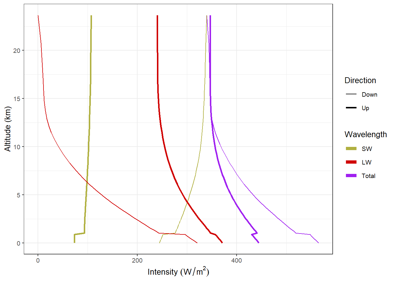
Figure 2: Upward and downward fluxes of longwave and shortwave radiation with low clouds.
We can see that for the low clouds, the biggest changes are in the downward flow of radiation. Downward longwave radiation is a lot greater below the clouds and downward shortwave is smaller. Above the clouds, there is a small increase in upward longwave and shortwave, but the changes are much smaller than for the downward radiation.
plot_heat_flows(high_clouds)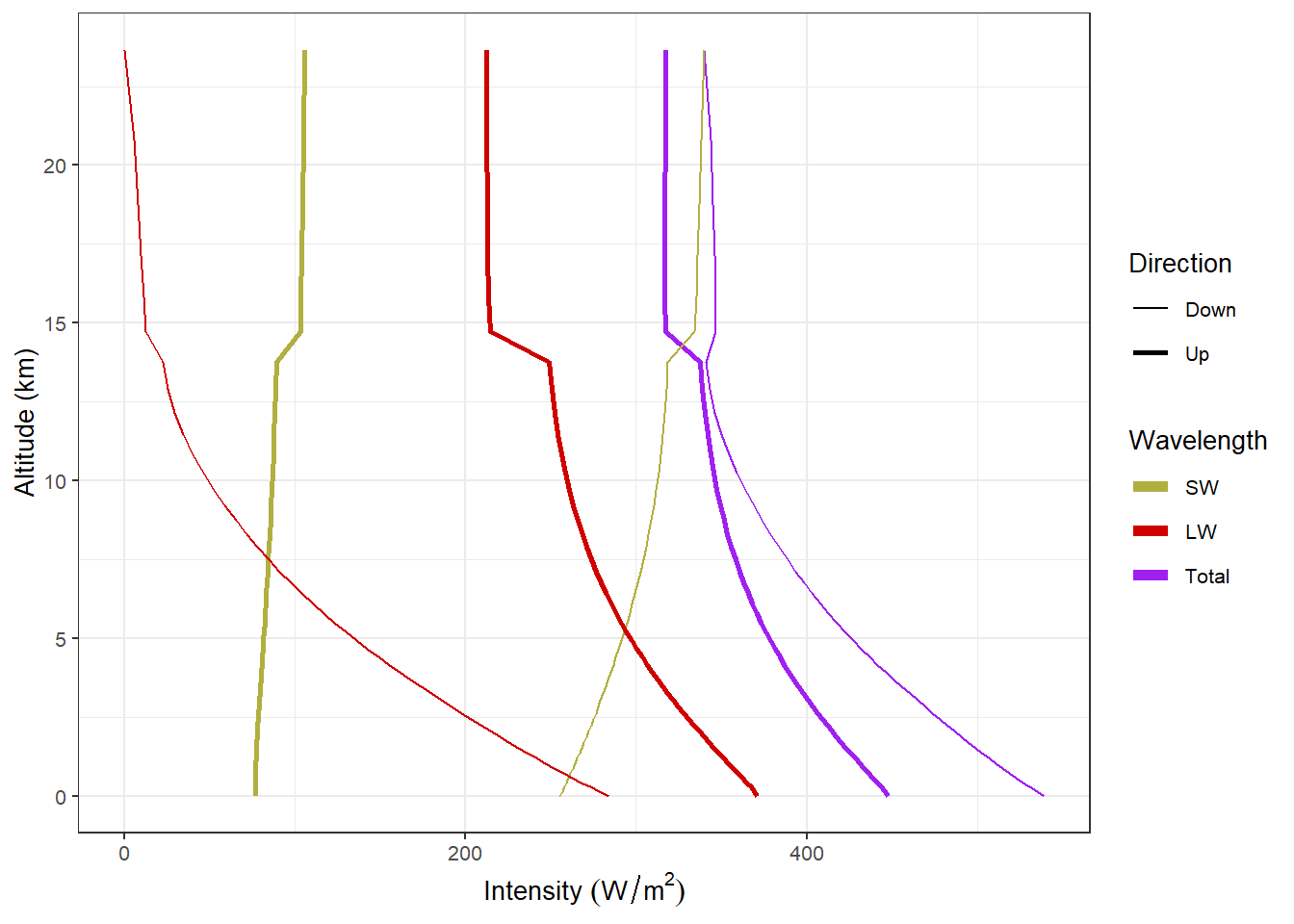
Figure 3: Upward and downward fluxes of longwave and shortwave radiation with high clouds.
At the height of the clouds we can see big changes in the upward radiation: Outgoing longwave radiation is considerably smaller above the clouds and outgoing shortwave is larger. There are changes to the downward radiation at the height of the clouds, but these changes are much smaller than for the upward radiation.
As these figures show, the low clouds had the greatest effect on downward radiation and the high clouds had the greatest effect on upward radiation. In both cases, the clouds affected the longwave radiation much more than the shortwave.
