EES 3310/5310

Reading for Lab #1 on Mon., Jan 24:

PDF version

Introduction to R and RMarkdown

RMarkdown

RMarkdown is a combination of two tools: Markdown is a simple way of writing plain text that can be formatted into fancy documents. Markdown originated as a tool for easily writing blog posts and comments that include formatting, such as section headings, italic and bold-faced text, and so forth without having to learn a technical formatting language, such as HTML. Markdown is fairly generic, so it is easy to translate a single Markdown document into many output formats, such as HTML for web pages, PDF, and Microsoft Word documents.

You can learn a lot about the details of Markdown at the RStudio web site http://rmarkdown.rstudio.com. RStudio has a handy cheat sheet for RMarkdown that you can see by opening the Help menu, going to “Cheatsheets” and opening the RMarkdown Cheat Sheet or the more comprehensive RMarkdown Reference.

What makes RMarkdown different from ordinary Markdown is that it allows you to combine text, formatted in Markdown, with instructions to the R statistical software to analyze data and produce graphs, tables, and other useful output.

By integrating the data analysis with the text of a document, we can easily make our research reproducible. The RMarkdown file contains all the instructions to load the data, analyze it, and generate the final report. Then if your data changes and you need to update your report, you can do so by knitting the RMarkdown document with the updated data files.

To turn an RMarkdown document into an HTML, PDF, or Microsoft Word document, you just click on the “Knit” button in RStudio. If you click on the word “Knit” on the button, RStudio will turn the RMarkdown document into the default format (see below). To knit the document into a different output format, click on the arrow just to the right of the word “Knit,” and select the output format you want.

I use RMarkdown to produce all of the documents I produce for the labs in this course. You can see my code at https://github.com/gilligan-ees-3310-2018. The code for all of the Lab #1 documentation is at https://github.com/gilligan-ees-3310-2018/lab_01_documentation

Breaking News: Markdown lets you use special characters in your text to specify the formatting (for example **this is boldface text** and _this is italic_ will become this is boldface text and this is italic), but the latest version of RStudio, which was released in January 2021, has a visual markdown editor that lets you edit Markdown the same way you’d edit text in a word processor and lets you see what the text will look like.

You can switch back and forth between the visual editor and the norrmal editor by clicking on the button on the top right of the editor pane that looks like the letter A.

Visual editor button in RStudio

Below I explain the structure of an RMarkdown document.

Document header

At the top of an RMarkdown document there is a section set off by lines of three hyphens above it and below it.

Here is an example:

---
title: "Your document's title"
subtitle: "Your document's subtitle"
author: "Your name goes here"
date: "Jan 24, 2022"
output:
    pdf_document: default
    html_document: default
---

By default, when RStudio knits the document, it converts it into the format listed first under output_format

When the output format lists, for instance, “pdf_format: default”, that means that when RStudio creates a pdf document, it uses the default options. If you want to customize the output, you can specify options for RStudio to use in creating PDF, HTML, or Word output documents:

---
title: "Your document's title"
subtitle: "Your document's subtitle"
author: "Your name goes here"
date: "Jan 24, 2022"
output:
    pdf_document:
      toc: "true" 
      number_sections: "false"
    html_document:
      self_contained: "false"
---

Markdown

Some of the basic elements of Markdown are:

Paragraphs

Any block of one or more lines of text, with a blank line before and a blank line after is treated as a single paragraph. To separate paragraphs, put a blank line between them:

Markdown:

This is one paragraph.
It stretches over several consecutive lines,
but it will be formatted 
as a single paragraph.

This is another paragraph.
The blank line between the two
blocks of text tells Markdown
that they are separate paragraphs

Formatted Output:

This is one paragraph. It stretches over several consecutive lines, but it will be formatted as a single paragraph.

This is another paragraph. The blank line between the two blocks of text tells Markdown that they are separate paragraphs

Section headers

Any line of text that begins with one or more hash symbols (“#”) and is preceded by a blank line is treated as a section header. Top-level section headers have a single hash, and subsections, subsubsections, etc. use two, three, etc. hashes.

Markdown:

# This is a top-level section header

## This is a subsection

### This is a subsubsection

# This is another section

Formatted Output:

This is a top-level section header

This is a subsection

This is a subsubsection

This is another section

Formatting text

To make italic text and boldface text you surround the text with underscores or asterisks. A single underscore or asterisk means italic, two means boldface, and three means both italic and boldface:

Markdown:

This is _italic text_. This is *also italic text*. __This is boldface__ and 
**so is this**. ***This is bold italic***. This is ~~strikethrough~~, perhaps 
to indicate an error.

Formatted Output:

This is italic text. This is also italic text. This is boldface and so is this. This is bold italic. This is ~~strikethrough~~, perhaps to indicate an error.

Lists

You can make bulleted or numbered lists easily in Markdown. Simply begin a line with an asterisk, hyphen, or plus sign. To make a sub-list, just indent the lines of the sublist by four spaces.

Markdown:

* This is a list

* This is the second item of the list.

    * This is a sub-list

    * This is another item in the sub-list
    
        A list item can have several paragraphs. Just ident the continuation 
        by four additional spaces and do not begin it with an asterisk.
        If you have multiple lines with no blank line separating them,
        Markdown treats them as a single paragraph.

        Here is a third paragraph of continuation.

* This is the main list again.
  Just as with other things, you can break a single list item into several lines,
  and as long as there is no blank line between them, Markdown knows to treat
  them as a single paragraph.

Formatted Output:

This is a list
This is the second item of the list.
- This is a sub-list
- This is another item in the sub-list
  
  A list item can have several paragraphs. Just indent the continuation by four additional spaces and do not begin it with an asterisk. If you have multiple lines with no blank line separating them, Markdown treats them as a single paragraph.
  
  Here is a third paragraph of continuation.
This is the main list again. Just as with other things, you can break a single list item into several lines, and as long as there is no blank line between them, Markdown knows to treat them as a single paragraph.

Numbered Lists

To make numbered lists, start them with a number and a period:

Markdown

1. This is a list

1. This is the second item of the list. Notice that I keep using the 
   numeral "1", but Markdown automatically increments the numbers
   for the list items.

    a) This is a sub-list

    a) This is another item in the sub-list
    
        A list item can have several paragraphs.
        
        Here is a third paragraph of continuation.
        
        i) this is a sub-sub list numbered with Roman numerals

        i) this is a sub-sub list numbered with Roman numerals

        i) this is a sub-sub list numbered with Roman numerals

1. This is the main list again.

Formatted Output:

This is a list
This is the second item of the list. Notice that I keep using the numeral “1”, but Markdown automatically increments the numbers for the list items.
1. This is a sub-list
2. This is another item in the sub-list
  
  A list item can have several paragraphs.
  
  Here is a third paragraph of continuation.
  1. this is a sub-sub list numbered with Roman numerals
  2. this is a sub-sub list numbered with Roman numerals
  3. this is a sub-sub list numbered with Roman numerals
This is the main list again.

Mathematical expressions

For simple math, you can just type stuff in RMarkdown: 1 + 2 * 3 comes out as 1 + 2 * 3. If you want subscripts or superscripts, you can get those by using the ~ and ^ characters, respectively: I~out~ = sigma T^4^ appears as I_out = sigma T⁴.

If you want fancier formatting for mathematical expressions, RMarkdown has a way to do this.

If you put an expression between dollar signs, RMarkdown interprets it differently from regular RMarkdown, and uses a format called LaTeX that is used for typesetting sophisticated mathematics. I won’t try to present all of LaTeX here, but will give some common examples:

An expression between single dollar signs is interpreted as in-line math that appears in the middle of a line of text. LaTeX uses special terms that begin with a backslash \ to indicate special mathematical formatting or operators. For example $a + b \times x$ appears as $a + b \times x$.

You can show Greek letters, like $\alpha$, $\pi$, and $\sigma$ by spelling them out like this: $\alpha$ , $\pi$ , and $\sigma$ . The epsilon that we use to indicate emissivity is a variation on the ordinary Greek epsilon, so we spell it $\varepsilon$ to get $\varepsilon$.

LaTeX handles subscripts and superscripts differently from RMarkdown: You use _{} and ^{} with whatever you want to appear in the subscript or superscript inside the braces {}: $I_{out} = \sigma T^{4}$ appears as $I_{out} = \sigma T^{4}$

You can include square root signs using \sqrt: $x = \sqrt{y \times z}$ appears as $x = \sqrt{y \times z}$. You can do other roots like this: $T = \sqrt[4]{I_{out} / \sigma}$ appears as $T = \sqrt[4]{I_{out} / \sigma}$.

To get display math, which appears on its own line, you use double dollar signs. This is useful when you want to write a mathematical expression that is much taller than a line of text. In display mode you can display fractions using \frac{numerator expression}{denominator expression}, as in this example: $$\varepsilon \sigma T^4 = \frac{(1 - \alpha)}{4} \times I_{solar}$$ appears as

\[ \varepsilon \sigma T^4 = \frac{(1 - \alpha)}{4} \times I_{solar}\] $$T_{bare rock} = \sqrt[4]{\frac{(1 - \alpha)}{4 \varepsilon \sigma} \times I_{solar}}$$ appears as

\[T_{bare rock} = \sqrt[4]{\frac{(1 - \alpha)}{4 \varepsilon \sigma} \times I_{solar}}\]

There is a lot more to the LaTeX notation that you can use in RMarkdown, but what I have shown here is sufficient for everything you will do in this class. You won’t need to use this kind of mathematical notation very much, but it can be convenient, especially when you are working exercises on atmospheric layer models.

If you find it too difficult to use LaTeX mathematical notation, I will accept either hand-written supplements in which you write out the equations by hand, or a textual description in your document where you use words instead of mathematical symbols to explain what you are doing.

Figures

You can include image files in your RMarkdown document:

Markdown

![This is a tornado](images/tornado.jpg)

Formatted Output:

This is a tornado

Hyperlinks

You can include links to documents on the web in two ways. The simplest is if you want the URL for the link to appear in your document you can just surround the URL with angle brackets: <https://www.vanderbilt.edu> appears as https://www.vanderbilt.edu.

If you want to add a hyperlink to some text in your document, then you would do it like this:

[Vanderbilt University](https://www.vanderbilt.edu)

to get this: Vanderbilt University.

Note the difference between the hyperlink specification and the image specification is whether there is an exclamation point before the square brackets.

Using R for calculations

RMarkdown combines the “Markdown” system for formatting text with the R statistical system for performing calculations and making graphs.

We are using R for the laboratory section of this course because it allows you to easily analyze large amounts of data and produce high-quality graphs.

To enter R expressions in an RMarkdown document, we use “code blocks” and “inline code”. Code blocks are useful if we are doing a calculation, and inline code is useful if you just want to insert a number (maybe one you have calculated in a code block) into the middle of a line of text.

Code blocks begin and end with three consecutive “back-tick” characters:

```{r code_block_name, options}
   # code goes here
```

Inline code appears between single back-ticks: `r code goes here`

We express basic mathematical operations in R similarly to the way we express them in Excel and most programming languages. Addition and subtraction use the normal plus and minus signs. Multiplication uses an asterisk, division uses a slash (“/”), and powers (exponentiation) uses “^”.

R has a lot of mathematical functions you can use, such as sqrt(), log() (for the natural logarithm), log10() for the base-10 logarithm, and so forth.

We can assign numbers to variables using the equals sign:

sigma = 5.67E-8
I_solar = 1350 # watts per square meter
albedo = 0.3
I_absorbed = I_solar * (1 - albedo)
T = (I_absorbed / (4 * sigma))^0.25

If the last line of a code block is something with a value (e.g., the name of a variable or a mathematical expression, as opposed to an assignment with an equals sign), then R will show that value:

## [1] 254.0664

We can also print the value of an R expression in the middle of a line of text using inline code: T = `r T` will give T = 254.0663741.

Inline code is very useful because it lets us ask R to automatically insert a number into the text. This means that every time we knit the document, that number is generated by R. If you write a report and then realize that there was a problem with the data or the analysis, you can just fix the problem and re-knit the report using the corrected data and analysis code. You don’t need to manually go through a separate document and edit the numbers to update them with the latest results from your analysis. RMarkdown will do that for you, if you used inline code to insert the numbers into your text.

Thus, a bit of extra work at the beginning to set up the document and analysis using RMarkdown saves lots of time later on by making it trivial to update the document.

Code blocks also allow us to include graphs in our document:

```{r graph_example, fig.cap = "This is a plot of pressure versus temperature."}
ggplot(pressure, aes(x = temperature, y = pressure)) +
  geom_line() +
  geom_point() +
  labs(x = "Temperature", y = "Pressure")
```

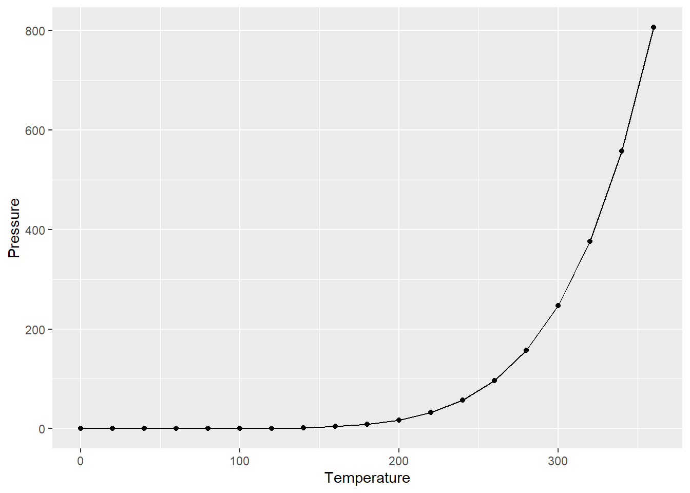
(#fig:graph_example)This is a plot of pressure versus temperature.

Loading R Scripts

In this course, I am trying to teach you to use the basics of R. Sometimes we will need to do things for our analysis that require more complicated R programming, and then I will write R scripts that contain this code so you don’t need to write it yourself from scratch, but can just call functions that I provide.

To load a script (a file containing R code), you use the R command source("script_file.R"")

For the exercises here, we will use two scripts, which are located in the “_scripts” directory.

To load them into R so you can use them in your analysis, you would put the following code into your RMarkdown document:

source("_scripts/format_md.R")
source("_scripts/layer_diagram.R")

Useful Scripts for the Labs:

These first script defines a function, format_md, which formats numbers nicely for markdown documents, allowing you to control how many significant digits it shows, and optionally using scientific notation or inserting commas to separate thousands, millions, etc.

format_md(sigma, digits = 1) will produce 0.000000057

format_md(pi * 1E6, digits = 3, format="scientific") will produce 3.142×10⁶

format_md(pi * 1E6, digits = 3, comma = TRUE) will produce 3,142,000

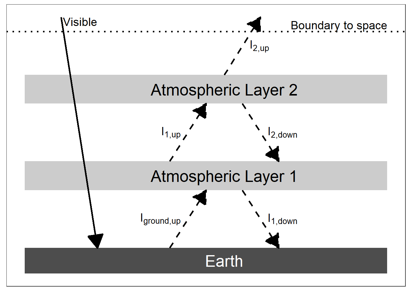
Script for Layer Diagrams

The other script allows you to produce a layer diagram, similar to the ones in Chapter 3 of Global Warming: Understanding the Forecast.

make_layer_diagram(2)