Reading for Lab #11 on Mon., Apr 11:
PDF version
New Tools for Data Analysis
Some New Tools for Working with Data
There are two new tools we will use in working with data for this lab:
Getting fancy with the pipe operator (%>%)
With the tidyverse, we often use the “pipe” operator %>% to send the
output from one function into the input of another function. In most cases,
this works very simply and it uses the output from the function on the
left as the first argument of the function on the right.
For instance, the filter function selects certain rows in a data frame or
tibble. I will work here with examples from the built-in storms data
frame that lists a subset of hurricanes from the National Oceanic and
Atmospheric Administration’s Atlantic hurricane database.
The data includes the positions and attributes of 198 tropical storms, measured
every six hours during the lifetime of the storm.
Let’s select Hurricane Katrina from 2005 (I specify the year because there were two earlier Katrinas in 1981 and 1999; storm names are re-used periodically unless they are retired because a storm with that name becomes historically important).
data(storms)
katrina = filter(storms, name == "Katrina", year == 2005)
and we can also do the same thing using the pipe operator like this:
storms %>% filter(name == "Katrina", year == 2005)What the pipe operator %>% does behind the scenes is take that output of
whatever is on the left (the data frame storms) and stick it in front
of the arguemnts for the function on the right so the two examples given
above are equivalent.
We have been usuing the pipe operator throughout the semester to combine
functions.
Suppose we want to mutate the storms data frame to add a new
column ts_area
that is equal to pi * (ts_diameter / 2)^2, where ts_diameter is a column
in storms that corresponds to the diameter (in nautical miles) of the area
in which winds are tropical storm strength or greater (36 knots),
and then we want to select only the data where the tropical storm area is
greater than 10,000 square nautical miles, and finally sort the data so the
rows of the data frame go from largest to smallest tropical storm area.
We can do that as follows:
# First way
df1 = arrange(filter(mutate(storms, ts_area = pi * (ts_diameter / 2.0)^2),
     ts_area > 10000), desc(ts_area))

# Second way, using a temporary variable
df2 = mutate(storms, ts_area = pi * (ts_diameter / 2.0)^2)
df2 = filter(df2, ts_area > 10000)
df2 = arrange(df2, desc(ts_area))

# Third way, using the pipe operator
df3 = storms %>% mutate(storms, ts_area = pi * (ts_diameter / 2.0)^2) %>%
     filter(ts_area > 10000) %>% arrange(desc(ts_area))
We use pipes because often they are simpler to understand. If we use the first way in the example above, if we are combining many functions, nesting functions inside other functions becomes very difficult to read and understand. The second way, of using temporary variables is fine, but it can get confusing to have lots of variable names that we use only one time to pass data from one function to another. The third way, using the pipe operator makes it easier to understand how the data is moving through the processing pipeline.
But the way pipe operators work can sometimes get in the way of things we want to do.
First, suppose that I want to send the results of a function into the second
or third argument of a subsequent function instead of the first argument?
We use the lm function to calculate the slope and intercept of a trend line
that best fits some data. The lm function expects the formula for the line
to fit to be the first argument and the data to be the second.
Suppose I want to examine hurricanes from the year 2005 and look for a relationship between the air pressure in the eye and the wind speed, but only during the time when they are classified as hurricanes.
I can do this as follows:
hurricanes_2005 = storms %>% filter(status == "hurricane", year == 2005)
lin_fit = lm(wind ~ pressure, data = hurricanes_2005)
The lm function looks at the data given by the data argument and
then finds the best line that characterizes the linear relationship
wind ~ pressure, which means that the wind is a linear function of the
pressure (this would be the slope of a graph where wind is on the y-axis
and pressure is on the x-axis).
Suppose that I would like to pipe data from the filter function to the
lm function. I have a problem because the pipe operator would put the
output from filter as the first argument of the lm function, but in
lm the first argument is the formula and data is the second.
I can do this as follows:
lin_fit2 = storms %>% filter(status == "hurricane", year == 2005) %>%
           lm(wind ~ pressure, data = .)
The pipe operator creates a new variable . (the period), which gets the
value of whatever is on the left of the operator. If I don’t use the .
in the function on the right, the pipe operator invisibly puts . in
the first argument so foo(x) %>% bar(y, z) is re-written behind the
scenes to become
. = foo(x)
bar(., y, z)
However, if I want to use the . somewhere else, I can do that explicitly
and when the pipe operator looks at the function on its right, it knows
not to stick the . in the first argument if I use . in the function
call. This, I could write foo(y) %>% bar(x, ., z) if I want to substitute
the output of foo(y) for the second argument of bar.
Extracting columns from a data frame in a pipeline
If I just want to look at the names of the hurricanes from the storms data
frame, I can use the $ operator:
names = storms$nameBut suppose that I want to filter the storms and then extract the names. What are the names of category 5 hurricanes?
cat_5 = storms %>% filter(category == 5)
names = cat_5$name
Suppose I want to do this without creating a variable cat_5?
I could try
# This will give an error
names = storms %>% filter(category == 5)$name
but it turns out that this doesn’t work because of the way the pipe operators
work.
To do this, I can use the pull function from the tidyverse:
# This will work
names = storms %>% filter(category == 5) %>% pull(name)
This will be useful for what comes next.
Tidying up results of statistical modeling
lm is one example of a lot of powerful functions in R that let you analyze
data by fitting models. A statistical model is an idealized functional relationship
between different attributes of the data (attributes are represented by columns
in a data frame).
For instance, a linear model idealizes two columns in the data frame in terms
of a linear relationship. For instance y~x represents a model in which
\(y = a + b x\). In fact, the data rarely lie exactly along a line, but
the lm function will find the values for a and b that define the line
that best relates y to x (specifically this will be the line such that
the minimizes the sum of the square of the errors between the actual y
and the line:
\(\sum_i (y_i - (a + b x_i))^2\).
We will be using lm in this lab to find the rates of change of different
parameters in the Kaya identity. For that we want to examine the slopes of the
lines identified by lm. We can do that as follows for the slope that relates
wind speed to pressure for a hurricane.
First, let’s plot the two variables to see wether there’s an apparent relationship. Let’s look at hurricanes from 2005:
storms %>% filter(status == "hurricane", year == 2005) %>%
  ggplot(aes(x = pressure, y = wind)) + geom_point(na.rm = T)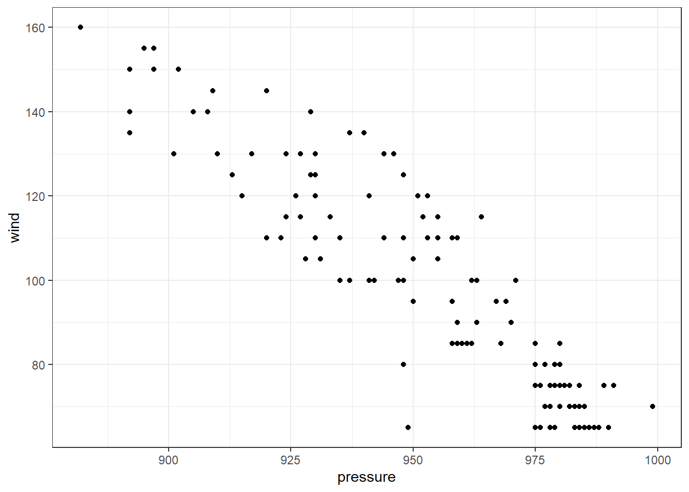
The data clearly doesn’t lie on a straight line, but there is a clear relationship that lower pressures tend to go along with higher wind speeds and higher pressures with lower wind speeds.
First, let’s review how we can fit a relationship between wind speed and pressure for hurricanes from 2005:
lin_fit = storms %>% filter(status == "hurricane", year == 2005) %>%
           lm(wind ~ pressure, data = .)
But how can we get the slope out of the variable lin_fit?
Here we use the broom package, which gives us a tidy function
that will tidy up the results of statistical models and put them
into a nice data frame:
lin_fit = storms %>% filter(status == "hurricane", year == 2005) %>%
           lm(wind ~ pressure, data = .)
tidy(lin_fit)
## # A tibble: 2 x 5
## term estimate std.error statistic p.value
## <chr> <dbl> <dbl> <dbl> <dbl>
## 1 (Intercept) 947. 25.3 37.4 5.07e-86
## 2 pressure -0.890 0.0263 -33.8 3.43e-79Here, term tells us the parameter: (Intercept) is the intercept
(a in the formula above), and pressure is the slope with respect to the
pressure (b in the formula above).
estimate is the estimate of the parameter (intercept or slope),
std.error is the uncertainty about the estimate of the parameter,
statistic and p.value are used for statistical hypothesis testing and we
will not use them so you can ignore them.
If I just want the slope, I can get that as follows:
lin_fit = storms %>% filter(status == "hurricane", year == 2005) %>%
           lm(wind ~ pressure, data = .)
slope = tidy(lin_fit) %>% filter(term == "pressure") %>% pull(estimate)
slope
## [1] -0.8896546Here, filter selects the row where term equals “pressure” and pull(estimate)
then selects the estimate column.
We can write this more compactly as follows:
slope = storms %>%
           filter(status == "hurricane", year == 2005) %>%
           lm(wind ~ pressure, data = .) %>%
           tidy() %>%
           filter(term == "pressure") %>% pull(estimate)
slope
## [1] -0.8896546Writing functions
If you are going to do the same calculation many times in R it is often useful to define a function that performs that calculation and then you can simply call the function whenever you want to do the calculation with new values.
For instance, in the “Growth Rates and Trends” section of the assignment for the bottom-up decarbonization lab, we see that if we have a quantity q that is growing at a steady percentage rate \(r_q\) each year and we know the value in one year \(y_0\) and want to predict what the value will be at a future year \(y\), we can calculate this as follows: \[ q(y) = q(y_0) \times \exp(r_q \times (y - y_0)). \] We can write this as an R function that we can call for different quantities and years:
growth = function(q_0, rate, start_year, end_year) {
  q_0 * exp(rate * (end_year - start_year))
}
A function definition has three parts:
First we have the name of the function (growth), then we have the word
function, followed by the arguments that the user must supply to the function
(q_0, rate, start_year, end_year), and then the body of the function, between
curly braces { ... }.
When you call the function, it executes all of the code between the curly braces
and returns the last value calculated before the closing brace.
Thus, we can call the function like this to estimate the world population
in 2050
P_2017 = 7.53 # world population was 7.53 billion
r_P = 0.0141  # growth rate is 1.41% per yer
P_2050 = growth(q_0 = P_2017, rate = r_P, start_year = 2017, end_year = 2050)
P_2050
## [1] 11.99146If you don’t specify the name of the parameter, the function fills them out in order, so we could also write
P_2017 = 7.53 # world population was 7.53 billion
r_P = 0.0141  # growth rate is 1.41% per yer
P_2050 = growth(P_2017, r_P, 2017, 2050)
P_2050
## [1] 11.99146kayadata: an R package for analyzing Kaya-identity data
You can install the kayadata package as follows:
library(devtools)
install_github("jonathan-g/kayadata")
or
library(pacman)
p_load_current_gh("jonathan-g/kayadata")
Once you have installed the kayadata package, you load it as follows:
library(kayadata)This package has several useful functions:
get_kaya_data(region_name): Get Kaya-identity data for a country or region.Argument:
region_nameis the name of the country or region you want data for (e.g., “United States”, “World”, “China”, etc.).You can inspect a list of countries and regions by running
kaya_region_list().- Results: The function returns a data frame with the following columns:
region: The country or region.year: The year.P: The population (in billions).G: The gross domestic product (in trillions).E: The primary energy consumption (in quads).F: The energy-related CO2 emissions (in millions of metric tons of CO2).g: Per-capita GDP (in thousands of dollars per person).e: The energy intensity of the economy (in quads per trillion dollars of GDP).f: The emissions intensity of the energy supply (in millions of metric tons of CO2 per quad).ef: The emissions intensity of the economy (in millions of metric tons of CO2 per trillion dollars of GDP).
- Results: The function returns a data frame with the following columns:
get_top_down_values(region_name): Get projections of the future values of Kaya-identity variables for a country, from the top-down International Energy Outlook analysis by the U.S. Energy Information Administration.- Argument:
region_nameis the name of the country or region you want data for (e.g., “United States”, “World”, “China”, etc.). - Results: The function returns a data frame with the following columns:
region: The country or region.year: The year (five-year intervals from 2015–2050).P: The population (in billions).G: The gross domestic product (in trillions).E: The primary energy consumption (in quads).F: The energy-related CO2 emissions (in millions of metric tons of CO2).g: Per-capita GDP (in thousands of dollars per person).e: The energy intensity of the economy (in quads per trillion dollars of GDP).f: The emissions intensity of the energy supply (in millions of metric tons of CO2 per quad).ef: The emissions intensity of the economy (in millions of metric tons of CO2 per trillion dollars of GDP).
- Argument:
get_top_down_trends(region_name): Get the trends for Kaya-identity variables for a country, from the top-down International Energy OUtlook analysis by the U.S. Energy Information Administration.- Argument:
region_nameis the name of the country or region you want data for (e.g., “United States”, “World”, “China”, etc.). - Results: The function returns a data frame with the following columns:
region: The country or regionP: The rate of change of the population (multiply by 100 to get the rate in percent per year).G: The rate of change of GDP.E: The rate of change of primary energy consumption.F: The rate of change of CO2 emissions.g: The rate of change of per-capita GDP.e: The rate of change of the energy intensity of the economy.f: The rate of change of the emissions intensity of the energy supply.ef: The rate of change of the emissions intensity of the economy.
- Argument:
project_top_down(region_name, year): Calculate projected values for Kaya identity variables at a future year from the present through 2050.- Arguments:
region_nameis the name of the country or region you want data for.year: The year you want projected data for (through 2050).- Results: A data frame with one row and columns for
region,year, and the Kaya variables: P, G, E, F, g, e, f, and ef.
- Arguments:
get_fuel_mix(region_name): Get the mixture of primary energy sources used by a country or region.- Argument:
region_nameis the name of the country or region you want data for (e.g., “United States”, “World”, “China”, etc.). - Results: The function returns a data frame with the following columns:
region: The country or regionregion_code: A three-letter code for the country or region.geography: The kind of region (“nation”, “region”, or “world”).year: The year the data represents.fuel: The kind of energy source (“Oil”, “Natural Gas”, “Coal”, “Nuclear”, “Hydro”, or “Renewables”)quads: The number of quads of that kind of energy consumed in that year.pct: The percent of total primary energy consumption that came from that kind of energy source.
- Argument:
plot_kaya(kaya_data, variable, start_year, stop_year, y_lab, log_scale, trend_line, points, font_size): Plot a time series showing trends in a Kaya variable.Arguments:
kaya_data: A data frame, like those returned byget_kaya_data.variable: A quoted Kaya variable name (“P”, “G”, “E”, “F”, “g”, “e”, “f”, or “ef”).start_year(optional): If you want to do trend analysis, you can specify the year to start calculating the trend. The graph will color the years fromstart_yeartostop_yearin a darker color.If you don’t specify
start_year, the default value is 1980. You can eliminate the special coloring and trend analysis by settingstart_year = NULL.stop_year(optional): The year to stop the trend analysis. If you don’t specifystop_year, it defaults to the last year in the data frame.y_lab(optional): The label for the y-axis. If you don’t specify this, R will pick an appropriate label based on which variable you choose.log_scale(optional): Set this toTRUEorFALSEto specify whether to plot the y-axis on a logarithmic scale. The default is to setlog_scale = FALSEif you don’t specify a value.trend_line(optional): Set this toTRUEorFALSEto specify whether to plot a trend line. The default is to settrend_line = FALSEif you don’t specify a value.points(optional): Set this toTRUEorFALSEto specify whether to plot points on the line. If you are making a small graph, the points may make the graph too busy. The default is to setpoints = TRUEif you don’t specify a value.font_size(optional): This lets you adjust the size of the fonts used in labeling the axes on the graph. If you are making small plots and the y-axis label won’t fit on the side of the graph, you might want to use a smaller font size. The default is to setfont_size = 20if you don’t specify a value.
Result: This function returns a plot object.
Example:
kd = get_kaya_data("World")
plot_kaya(kd, "F")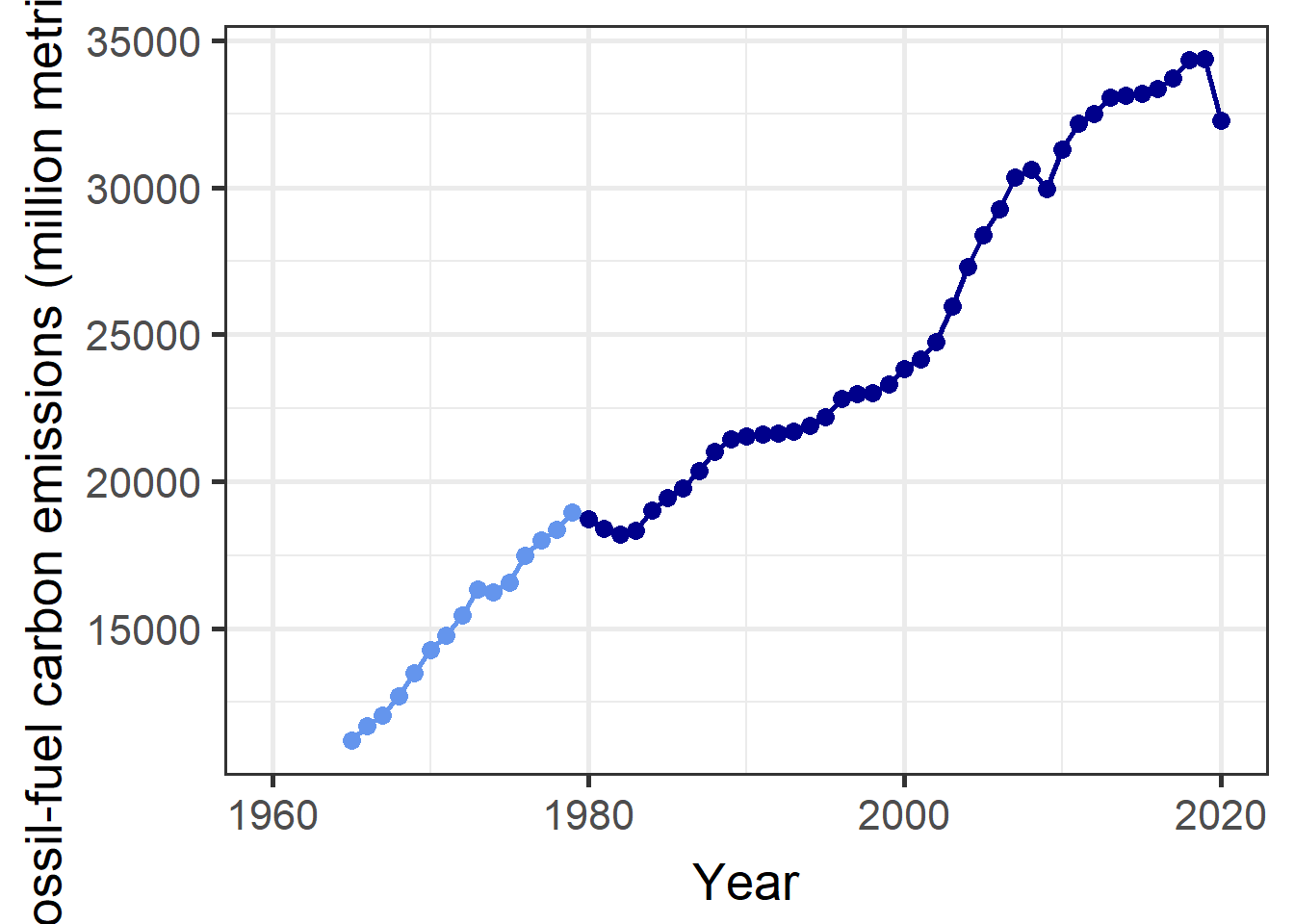
plot_kaya(kd, "F", log_scale = TRUE, font_size = 12, trend_line = TRUE)
plot_kaya(kd, "F", points = FALSE, start_year = NULL, font_size = 12)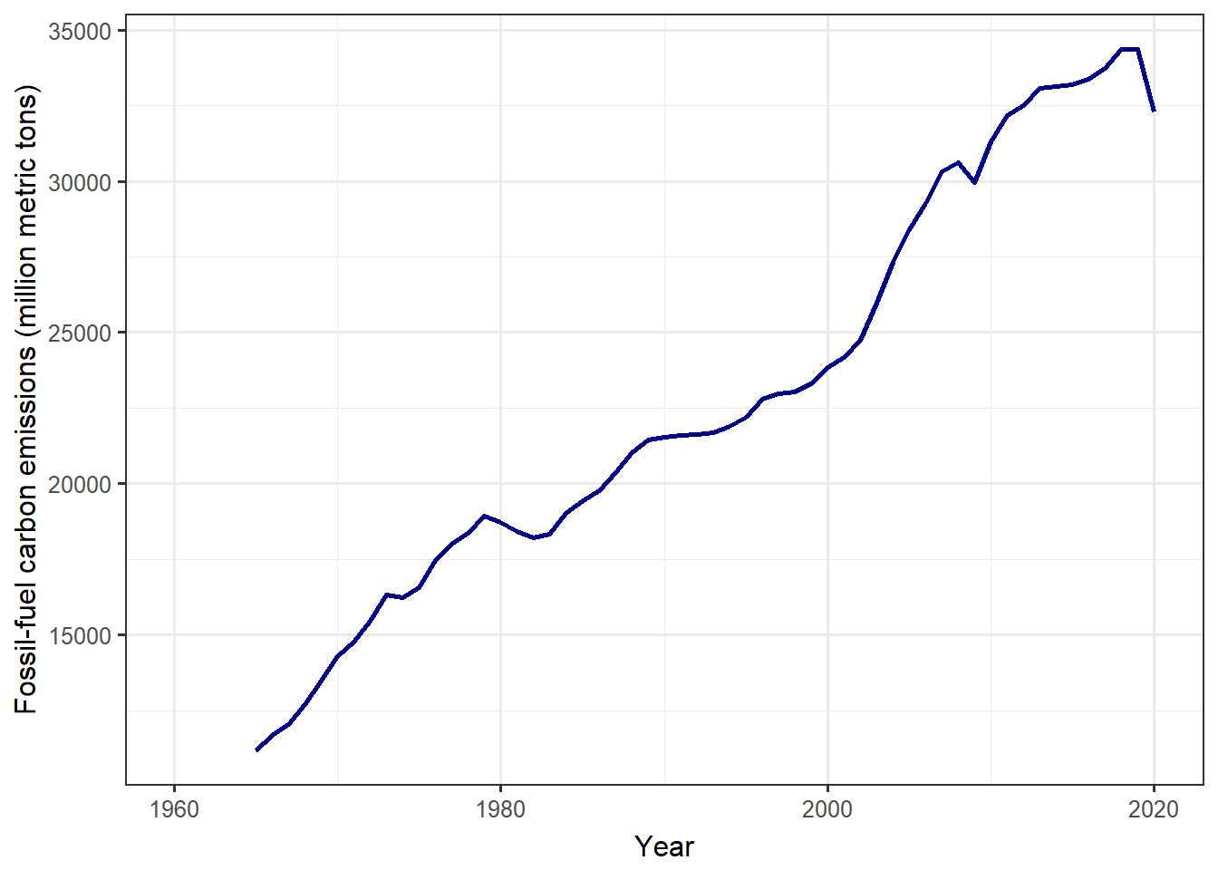
plot_fuel_mix(fuel_mix, collapse_renewables): Make a “donut” chart showing the amount of energy the country got from different energy sources.- Arguments:
fuel_mix: A data frame with the fuel mix for the country, like the ones returned byget_fuel_mix()collapse_renewables(optional): Set this toTRUEorFALSEto specify whether to combine “Hydro” with other renewables to make one “Renewables” category (TRUE), or plot “Hydro” separately from the other renewables (FALSE).If you don’t specify
collapse_renewables, the default is to setcollapse_renewables = TRUE. Settingcollapse_renewables = FALSEwill only work if you also specifiedcollapse_renewables = FALSEwhen you retrieved the fuel mix usingget_fuel_mix().Results: A plot object with a donut chart.
Example:
fm = get_fuel_mix("World")
plot_fuel_mix(fm)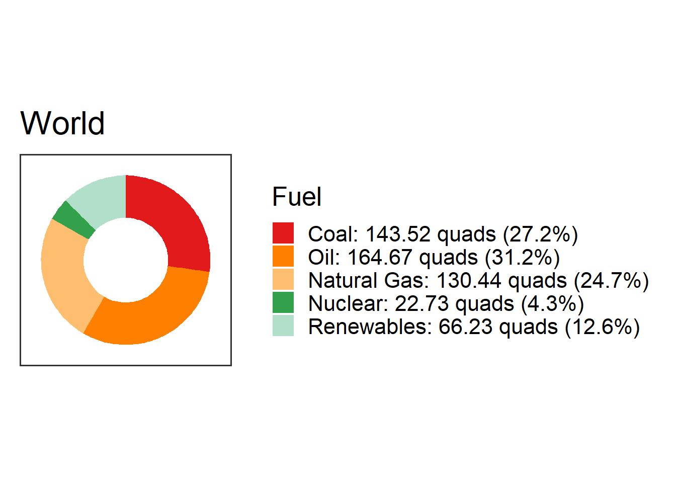
fm = get_fuel_mix("World", collapse_renewables = FALSE)
plot_fuel_mix(fm, collapse_renewables = FALSE)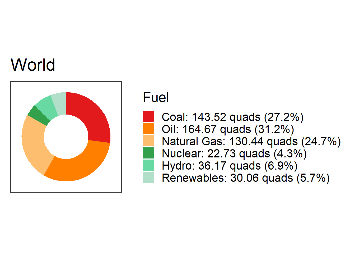
- Arguments:
kaya_region_list(): Get a list of regions and countries for which you can get Kaya data.emissions_factors(): Get a data frame with columns forfuel: The energy sourceemission_factor: The emissions from that energy source, in million metric tons of CO2 per quad of energy.
generation_capacity(): Get a data frame with generation capacity of a typical power plant for different kinds of energy sources. This data frame has columns:fuel: The energy source.description: A description of the kind of power plant.nameplate_capacity: The “nameplate capacity” of a typical power plant of that type. The nameplate capacity is the power output when the plant is running at its maximum capacity.capacity_factor: The capacity factor. This is the fraction of the nameplate capacity that the power plant can produce over an average year.The average power output from a power plant is the nameplate capacity times the capacity factor: \[ \text{average power} = \text{nameplate capacity} \times \text{capacity factor} \]
