Lab #5 Lab #5 Answers
PDF version
Lab #5 Answers
In the answers below, I illustrate how you can use RMarkdown to integrate code and data analysis with your text to produce a clear report that follows the principles of reproducible research
Exercise 1: Clouds and Infrared.
Clouds play an important and complex role in the climate system because they interact with both visible and infrared light. In this exercise, I investigated the way that the clouds interact with the flow of heat in the form of longwave infrared light.
I began by comparing the longwave radiation going out from the atmosphere to space under four conditions: with no clouds and with low, medium, and high-altitude clouds. Next, I compared the upward longwave radiation going out to space with the radiation going downward from the atmosphere, which is absorbed by the surface, and compared the upward and downward radiation for clear skies and with low clouds. Finally, I investigated the effect of water vapor on the downward radiation, which let me compare the impact of water vapor to the impact of clouds.
The earth’s temperature is determined by balancing incoming and outgoing radiation. Incoming radiation reaches the earth as shortwave radiation from the sun and for this lab, I will only look at the effect clouds have on longwave radiation, so I will ignore the way clouds affect shortwave radiation (i.e., I will ignore the way that clouds change the earth’s albedo).
Clouds and Outgoing Longwave Radiation
First, I look at the effect clouds have on outgoing radiation. To do this, I start by running MODTRAN with the default settings, which include a clear sky with no clouds:
default_outgoing = run_modtran(atmosphere = "tropical", altitude_km = 70,
                               looking = "down")
i_out_clear = default_outgoing$i_out
plot_modtran(default_outgoing, descr = "Clear sky, looking down from 70 km")
## colors = (MODTRAN = black, 300 K = #CC1414, 280 K = #A7CC14, 260 K = #14CC5E, 240 K = #145ECC, 220 K = #A714CC)## linetypes = (MODTRAN = solid, 300 K = 44, 280 K = 84, 260 K = 88, 240 K = 26, 220 K = 2686)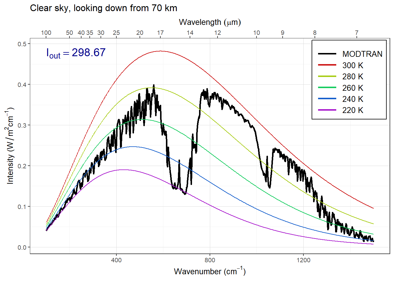
(#fig:modtran_default)Looking down from 70 km with a clear sky.
Next, I do the same for three kinds of clouds: low-altitude stratus clouds, medium altitude altostratus, and high-altitude cirrus.
stratus_outgoing = run_modtran(atmosphere = "tropical", altitude_km = 70,
                               looking = "down", clouds = "stratus")
altostratus_outgoing = run_modtran(atmosphere = "tropical", altitude_km = 70,
                               looking = "down", clouds = "altostratus")
cirrus_outgoing = run_modtran(atmosphere = "tropical", altitude_km = 70,
                               looking = "down", clouds = "standard cirrus")

i_out_stratus = stratus_outgoing$i_out
i_out_altostratus = altostratus_outgoing$i_out
i_out_cirrus = cirrus_outgoing$i_out
plot_modtran(stratus_outgoing,
descr = "Stratus clouds, looking down from 70 km")## colors = (MODTRAN = black, 300 K = #CC1414, 280 K = #A7CC14, 260 K = #14CC5E, 240 K = #145ECC, 220 K = #A714CC)## linetypes = (MODTRAN = solid, 300 K = 44, 280 K = 84, 260 K = 88, 240 K = 26, 220 K = 2686)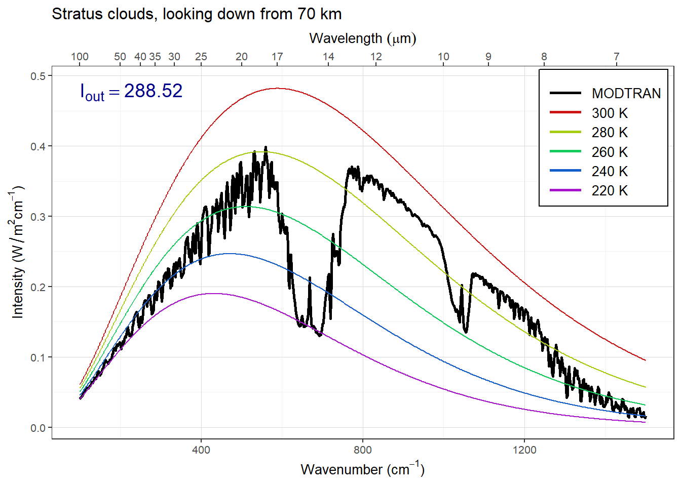
Figure 1: Looking down on stratus clouds from 70 km
plot_modtran(altostratus_outgoing,
                         descr = "Altostratus clouds, looking down from 70 km")
## colors = (MODTRAN = black, 300 K = #CC1414, 280 K = #A7CC14, 260 K = #14CC5E, 240 K = #145ECC, 220 K = #A714CC)## linetypes = (MODTRAN = solid, 300 K = 44, 280 K = 84, 260 K = 88, 240 K = 26, 220 K = 2686)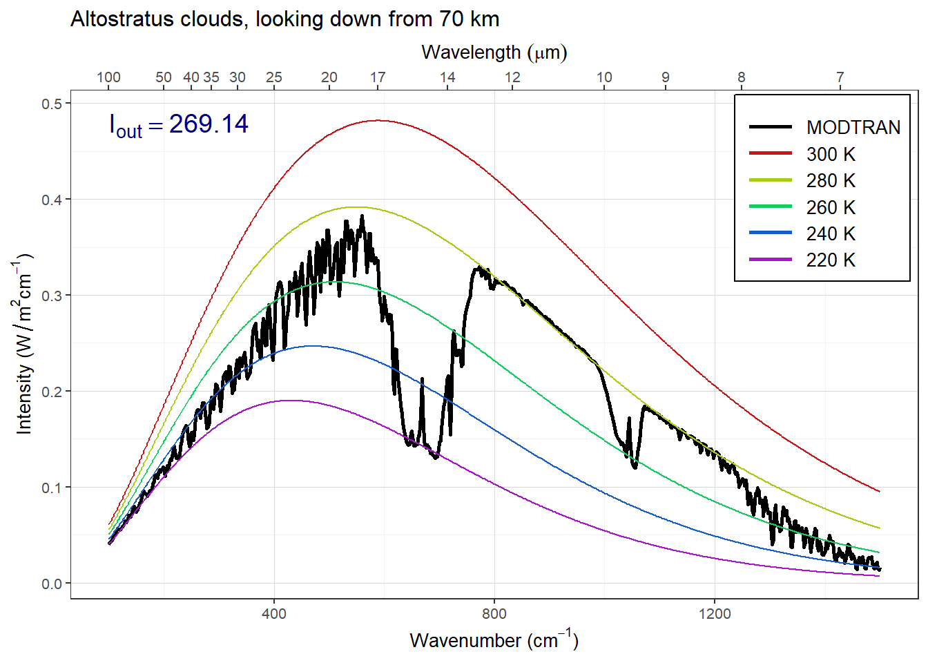
Figure 2: Looking down on altostratus clouds from 70 km
plot_modtran(cirrus_outgoing,
                         descr = "Cirrus clouds, looking down from 70 km")
## colors = (MODTRAN = black, 300 K = #CC1414, 280 K = #A7CC14, 260 K = #14CC5E, 240 K = #145ECC, 220 K = #A714CC)## linetypes = (MODTRAN = solid, 300 K = 44, 280 K = 84, 260 K = 88, 240 K = 26, 220 K = 2686)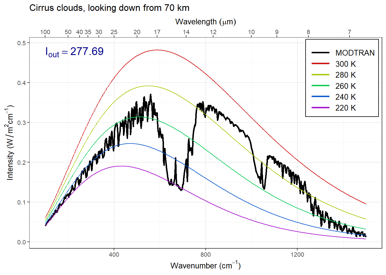
Figure 3: Looking down on cirrus clouds from 70 km
The following table compares the total intensity of outgoing radiation with different kinds of clouds and with a clear sky:
i_out_tbl = tibble(clouds = c("none", "stratus", "altostratus", "cirrus"),
                   altitude = c("", "low", "medium", "high"),
                   i_out = c(i_out_clear, i_out_stratus, i_out_altostratus,
                             i_out_cirrus),
                   change = i_out - i_out_clear
                   )
kable(i_out_tbl, digits = 1)| clouds | altitude | i_out | change |
|---|---|---|---|
| none | 298.7 | 0.0 | |
| stratus | low | 288.5 | -10.1 |
| altostratus | medium | 269.1 | -29.5 |
| cirrus | high | 277.7 | -21.0 |
Adding stratus (low-altitude) clouds reduces Iout by 10.1 W/m2, adding cirrus (high-altitude) clouds reduces Iout by 21.0W/m2, and altostratus (medium-altitude) clouds reduces Iout by 29.5W/m2.
When we compare the spectra of outgoing radiation, there is very little difference in the parts of the spectrum where greenhouse gases absorb strongly (CO2 near 700 cm-1, ozone near 1050 cm-1, and water vapor in the regions below about 550 cm-1 and above 1200 cm-1), but there are clear differences in the two atmospheric window regions (800–1000 cm-1 and 1100–1200 cm-1), where the greenhouse gases do not absorb very much. For all three cloud types, the outgoing radiation is smaller in both window regions. The difference is greatest for altostratus, less for cirrus, and least of all for stratus.
What is happening here is the radiation we see with clear skies in the window region is coming from the very low atmosphere, near the surface. When there are clouds, they are higher up, so they block the radiation from near the surface, but they also emit radiation at an intensity that corresponds to the temperature of the tops of the clouds.
The higher up you go, the colder the temperature is, so the cold tops of the clouds emit longwave radiation with lower intensity than the atmosphere below them would.
The difference between stratus and altostratus has to do with the altitude of the clouds: higher altitudes correspond to lower temperatures, so the tops of altostratus clouds (medium altitude) are colder than the tops of the stratus clouds (low-altitude).
With cirrus, the situation is more complicated. Stratus and altostratus clouds tend to cover the whole sky, but cirrus clouds are wispy and only cover a small fraction of the sky (see the pictures from my lecture for class #8 on Feb. 10: https://ees3310.jgilligan.org/slides/class_08/#/cloud-feedbacks-2 and https://ees3310.jgilligan.org/slides/class_08/#/cloud-feedbacks-3). This means that the cirrus clouds will have a smaller effect on outgoing radiation than the altostratus clouds, even though their temperature is lower. (Note: Students do not need to get the explanation of cirrus clouds correct to get full credit for this exercise.)
Looking up from the Ground with a Clear Sky
We have spent a lot of time looking down from high in the atmosphere, but MODTRAN also lets us look up from the ground and see the longwave light coming down to the surface from the atmosphere. We start by comparing the spectrum of longwave radiation going up to space and going down to the surface under a clear sky:
clear_up = run_modtran(atmosphere = "midlatitude winter",
                         altitude_km = 70, looking = "down",
                         h2o_scale = 1, clouds = "none")
plot_modtran(clear_up, descr = "Looking down from 70 km with clear skies")
## colors = (MODTRAN = black, 300 K = #CC1414, 280 K = #A7CC14, 260 K = #14CC5E, 240 K = #145ECC, 220 K = #A714CC)## linetypes = (MODTRAN = solid, 300 K = 44, 280 K = 84, 260 K = 88, 240 K = 26, 220 K = 2686)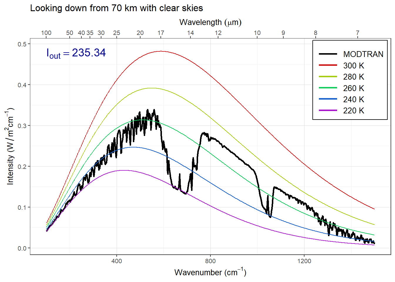
Figure 4: Upward longwave radiation going out to space from a clear sky
clear_down = run_modtran(atmosphere = "midlatitude winter",
                         altitude_km = 0, looking = "up",
                         h2o_scale = 1, clouds = "none")
i_down_clear = clear_down$i_out
plot_modtran(clear_down, descr = "Looking up from 0 km with clear skies")
## colors = (MODTRAN = black, 300 K = #CC1414, 280 K = #A7CC14, 260 K = #14CC5E, 240 K = #145ECC, 220 K = #A714CC)## linetypes = (MODTRAN = solid, 300 K = 44, 280 K = 84, 260 K = 88, 240 K = 26, 220 K = 2686)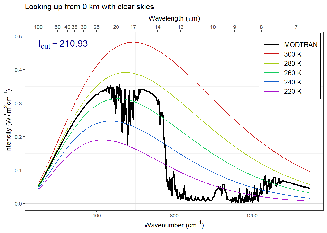
Figure 5: Downward longwave radiation coming to the surface from a clear sky
When we compare the two spectra, they are almost opposite. The upward radiation going out to space is brightest in the atmospheric window and dimmest where CO2 absorbs strongly. The downward radiation reaching the ground is brightest where CO2 and water vapor absorb strongly and dimmest in the atmospheric window.
The reason for this is that where the atmosphere is most transparent, a lot of the radiation we see is coming from whatever is on the other side of the atmosphere. When we are on the surface looking up with our eyes, and we aren’t looking at the sun we see visible light from space (the moon and stars). Outer space is very cold, so in the atmospheric window region of the longwave spectrum, our sensor looking up from the surface sees blackbody radiation corresponding to the cold temperatures of space, and our sensor looking down from 70 km sees blackbody radiation corresponding to the warm temperature of the surface.
Where CO2 absorbs strongly, when we look down from space, the CO2 in the atmosphere absorbs the bright radiation from the warm lower atmosphere before it can get up to the sensor, so what we see is the blackbody radiation from CO2 molecules high up in the atmosphere where the temperature is cold, so the radiation is very faint. When we look up from the surface, CO2 molecules near the surface have high emissivity, so they radiate strongly and the sensor sees intense radiation. The same applies to water vapor, and the sensor sees bright, intense radiation in the parts of the spectrum where water vapor absorbs strongly (i.e., where it has a large emissivity).
Looking up from the Ground with Clouds
Next, I investigated how the presence of clouds changes the spectrum that a sensor looking up from the ground will see.
stratus_down = run_modtran(atmosphere = "midlatitude winter",
                         altitude_km = 0, looking = "up",
                         h2o_scale = 1, clouds = "stratus")
i_down_stratus = stratus_down$i_out
plot_modtran(stratus_down, descr = "Looking up from 0 km with stratus clouds")
## colors = (MODTRAN = black, 300 K = #CC1414, 280 K = #A7CC14, 260 K = #14CC5E, 240 K = #145ECC, 220 K = #A714CC)## linetypes = (MODTRAN = solid, 300 K = 44, 280 K = 84, 260 K = 88, 240 K = 26, 220 K = 2686)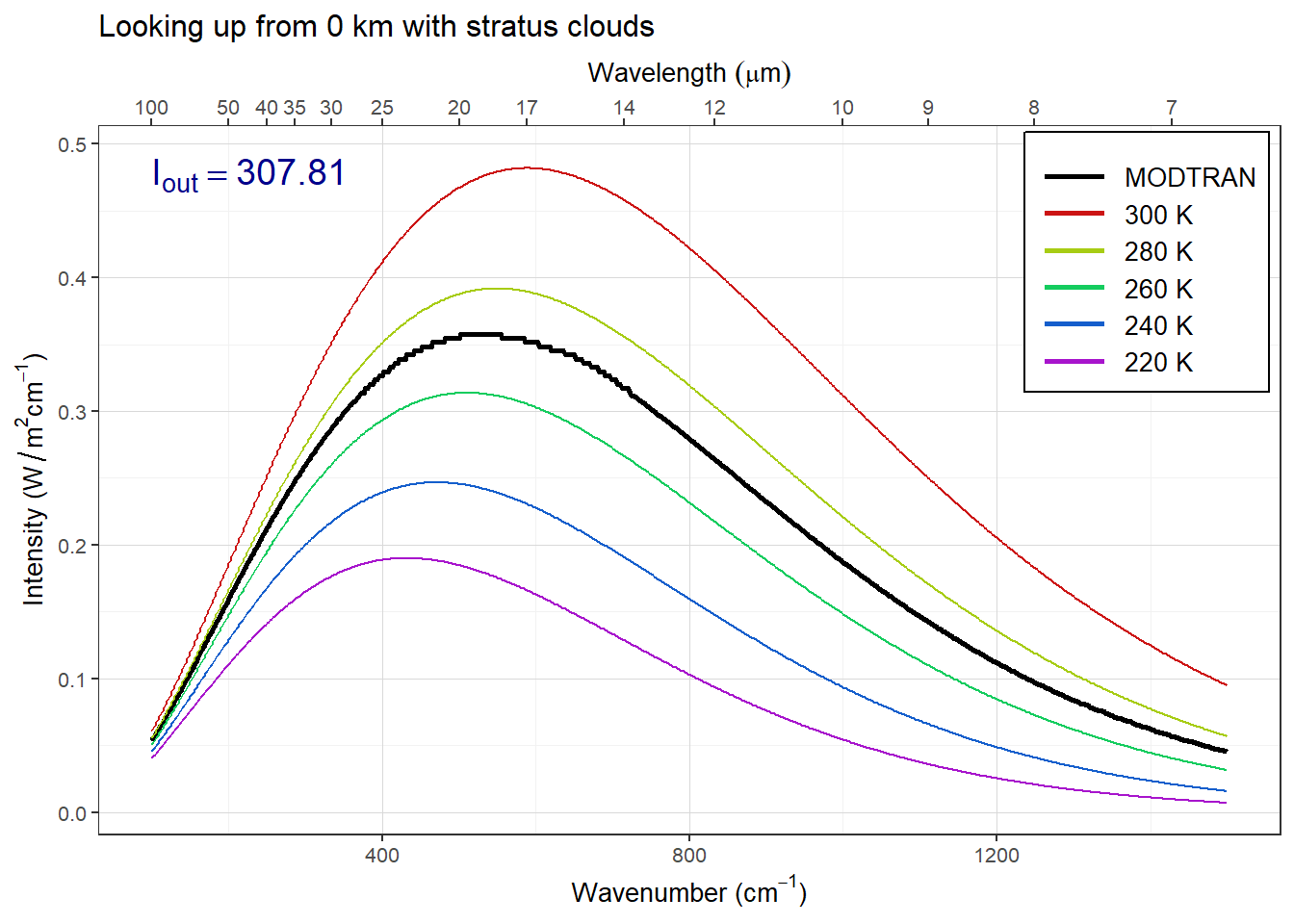
Figure 6: Downward longwave radiation coming to the surface from stratus clouds
Here, the spectrum looks like a perfect black body at a temperature of around 270 K. The bottom of the cloud acts like a perfect blackbody, and stratus clouds are low in the sky, so the temperature is relatively high. This has an especially big effect in the atmospheric window regions of the spectrum. In the windows, the downward spectrum was very faint with clear skies, but with stratus clouds the windows have a lot of downward radiation.
Basically, the bottoms of the low clouds are warm, and because of this, they glow brightly with longwave blackbody radiation, and that sends a lot of heat to the surface. Adding stratus clouds to a winter sky increased the heat coming to the surface from the atmosphere from 210.9 Watts per square meter under clear skies to 307.8 Watts per square meter.
This extra heat will warm the ground, so on a winter night, we expect the temperature to be a good deal warmer when the sky is cloudy than when it is clear.
The Effect of Water Vapor
Next, I investigated the way water vapor affects outgoing longwave radiation and compare that to the effects of clouds. To do this, I compare the intensity of downward longwave radiation at the surface with the normal amount of water vapor in the atmosphere to the intensity when there is no water vapor.
The previous clear-sky run had a normal amount of water vapor, so I only need to
run MODTRAN with h2o_scale = 0 and compare that to the previous clear_down
run, which had the default value h2o_scale = 1
dry_down = run_modtran(atmosphere = "midlatitude winter",
                         altitude_km = 0, looking = "up",
                         h2o_scale = 0, clouds = "none")
i_down_dry = dry_down$i_out
plot_modtran(dry_down,
             descr = "Looking up from 0 km with a clear sky and no water vapor")
## colors = (MODTRAN = black, 300 K = #CC1414, 280 K = #A7CC14, 260 K = #14CC5E, 240 K = #145ECC, 220 K = #A714CC)## linetypes = (MODTRAN = solid, 300 K = 44, 280 K = 84, 260 K = 88, 240 K = 26, 220 K = 2686)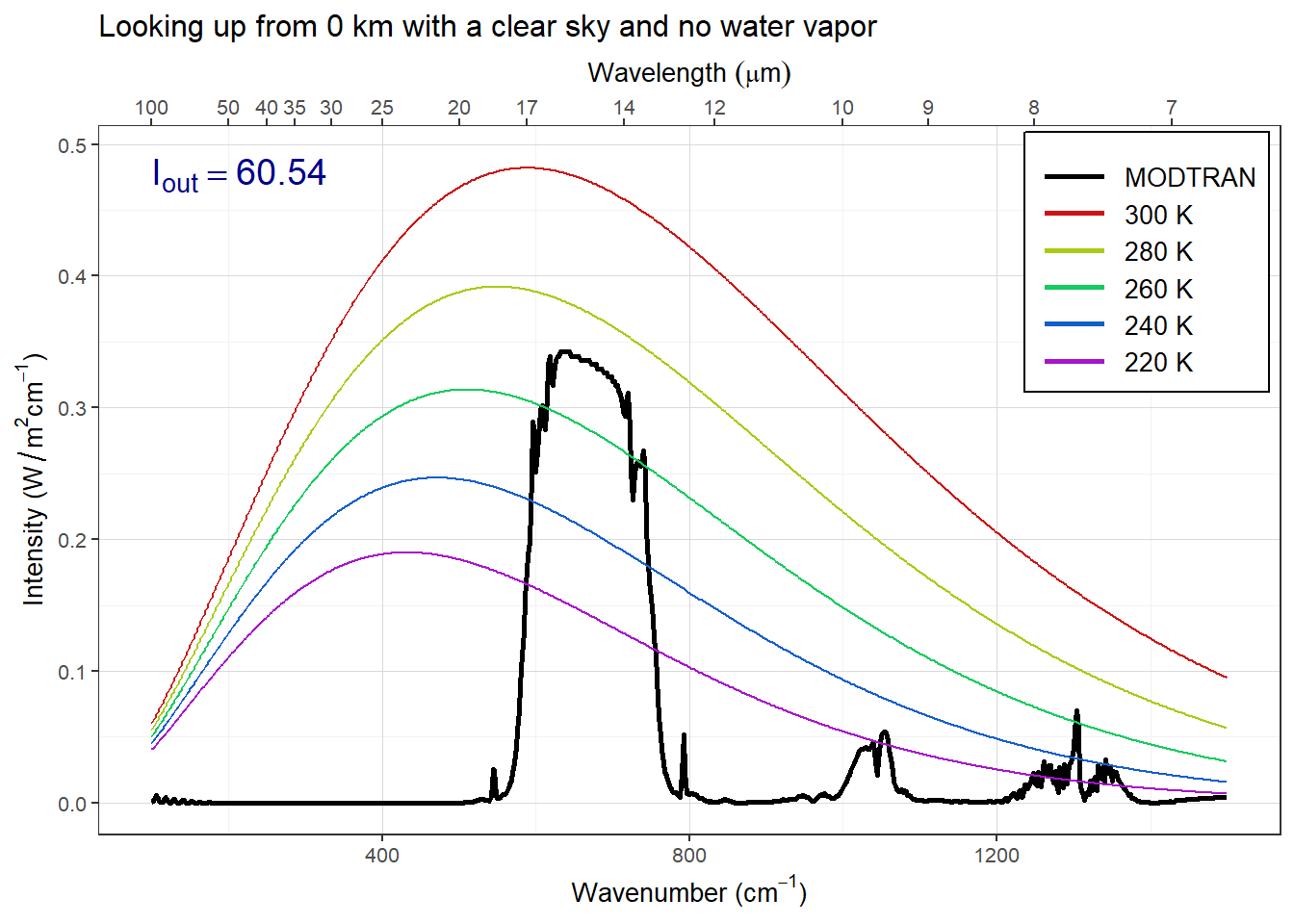
Figure 7: Downward longwave radiation coming to the surface with a clear sky and no water vapor
This spectrum contrasts dramatically with the spectrum of downward radiation for clear skies with a normal amount of water vapor. In the regions below about 550 cm-1 and above 1200 cm-1, the longwave radiation is much less intense—indeed, there is basically none, except for the region around 1300 cm-1 where methane absorbs and emits.
The three big features of longwave emission correspond to the CO2 absorption near 700 cm-1, ozone absorption near 1050 cm-1, and methane absorption near 1300 cm-1. Other than those three features, there is essentially no downward radiation. This is because without any water vapor, the atmosphere is mostly transparent to longwave radiation, and because good absorbers are also good emitters, this means that the amosphere emits almost no radiation in most of the spectrum. What the sensor sees from the ground in most of the spectrum is just the cold temperature of space, and the correspondingly low intensity of longwave radiation.
The total downward radiation with clear skies and no water vapor is 60.5 W/m2, which is 150.4 W/m2 less than for clear skies with water vapor. This difference is a way to measure the greenhouse effect of water vapor: adding water vapor to the atmosphere increases the amount of heat absorbed by the surface by 150.4 W/m2. This heat is longwave radiation emitted by the water vapor in the atmosphere, and it heats up the earth’s surface (the ground and the water at the surface of the oceans).
Water vapor has a much larger effect than adding clouds. Adding stratus clouds to a clear sky increased Iout by 96.9 W/m2 and adding water vapor to a dry atmosphere increased Iout by 150.4 W/m2.
Exercise 2: Water Vapor Feedback
In the previous exercise I found that water vapor affects longwave radiation very powerfully. The amount of water vapor in the atmosphere depends on the air temperature. The warmer the air is, the more water vapor it can hold, so as temperatures rise, the amount of water vapor also rises, and as temperatures fall, the amount of water vapor falls. This effect creates a powerful positive feedback involving water vapor.
Here I will estimate the effect of the water-vapor feedback using the RRTM climate model, which includes the effects of both radiation and convection. To measure the water vapor feedback, I will measure the climate sensitivity under normal conditions and when there is no water vapor in the atmosphere.
Finding the Climate Sensitivity
The climate sensitivity is defined as the change in surface temperature that occurs when the amount of CO2 is doubled. To calculate the climate sensitivity with the RRRTM model, I first ran the model with CO2 at its current value of 440 ppm, and make sure that the heat flow into and out of the earth is balanced. Then I ran the model with CO2 doubled to 800 ppm and adjusted the surface temperature until the model reported that the heat flow was balanced.
First, I ran the RRTM model with its default parameters.
rrtm_default = run_rrtm(co2_ppm = 400, relative_humidity = 80)
q_default = rrtm_default$Q
The results from RRTM model runs include the variable Q, which is the imbalance of Iin - Iout, so if Q > 0, there is more heat coming in and the earth will warm up, and if Q < 0, there is more heat going out and the earth will cool off.
Here, I can verify that the RRTM model in its default configuration has Q = 0 W/m2.
Next, I ran RRTM with CO2 doubled:
rrtm_doubled = run_rrtm(co2_ppm = 800, relative_humidity = 80)
q_doubled = rrtm_doubled$Q
With CO2 doubled, Q becomes 4.2 W/m2. Using trial and error with the interactive web version of RRTM, I found a temperature where Q = 0. Initially, Q was 4.2, which is greater than 0, so I knew that I had to increase the surface temperature. I first raised the surface temperature from 284.4 K to 290 K.
test_T_1 = 290
rrtm_test_1 = run_rrtm(co2_ppm = 800, relative_humidity = 80,
                       T_surface = test_T_1)
q_test_1 = rrtm_test_1$Q
Now, Q = -5.1, which is less than zero, so I needed to reduce Tsurface. I chose a value roughly halfway between the original temperature (284.4 K) and 290 K: my new guess was 287 K.
test_T_2 = 287
rrtm_test_2 = run_rrtm(co2_ppm = 800, relative_humidity = 80,
                       T_surface = test_T_2)
q_test_2 = rrtm_test_2$Q
Now, Q = -0.20, which is still slightly less than zero, so I needed to reduce Tsurface a bit more. I chose a value roughly halfway between the original temperature (284.4 K) and 287 K: my new guess was 286 K
test_T_3 = 286
rrtm_test_3 = run_rrtm(co2_ppm = 800, relative_humidity = 80,
                       T_surface = test_T_3)
q_test_3 = rrtm_test_3$Q
Now, Q = 1.5, so I guess a new temperature halfway between 286 and 287
test_T_4 = 286.5
rrtm_test_4 = run_rrtm(co2_ppm = 800, relative_humidity = 80,
                       T_surface = test_T_4)
q_test_4 = rrtm_test_4$Q
Now, Q = 0.70, so I guess a new temperature halfway between 286.5 and 287
test_T_5 = 286.75
rrtm_test_5 = run_rrtm(co2_ppm = 800, relative_humidity = 80,
                       T_surface = test_T_5)
q_test_5 = rrtm_test_5$Q
Now, Q = 0.20, so I guess a new temperature halfway between 286.75 and 287
test_T_6 = 286.87
rrtm_test_6 = run_rrtm(co2_ppm = 800, relative_humidity = 80,
                       T_surface = test_T_6)
q_test_6 = rrtm_test_6$Q
Now, Q = 0, so I am done and the new equilibrium surface temperature is 286.87. The climate sensitivity for an atmosphere with 80% average humidity is the change in surface temperature that was necessary to bring Q to zero.
climate_sensitivity_humid = test_T_6 - rrtm_doubled$T_surfaceThe climate sensitivity is 2.45 K
Climate Sensitivity without Water Vapor
Next, I do the same exercise, but with relative_humidity = 0 so there will be
no water-vapor feedback.
First, I run RRTM with no water vapor and 400 ppm CO2:
rrtm_dry = run_rrtm(co2_ppm = 400, relative_humidity = 0)
q_dry = rrtm_dry$QQdry = -91., so before I can do anything else, I need to adjust Tsurface to bring Q to zero.
new_T_surface = 261.55
rrtm_dry_eq = run_rrtm(co2_ppm = 400, relative_humidity = 0,
                       T_surface = new_T_surface)
q_dry_eq = rrtm_dry_eq$Q
Repeating the same trial-and-error process illustrated above, I tried Tsurface = 270 K, then 260 K, then 265 K, then 262.5 K, then 261 K, then 261.5 K, then 261.6 K, then 261.55 K, which finally gave Q = 0.
Next, I doubled CO2
rrtm_doubled_dry = run_rrtm(co2_ppm = 800, relative_humidity = 0,
                            T_surface = new_T_surface)
q_doubled_dry = rrtm_doubled_dry$QQdoubled,dry = -91., so before I can do anything else, I need to adjust Tsurface to bring Q to zero.
After some trial and error, similar to what I showed above, I found that raising the surface temperature by 1.1 K would bring Q to 0
climate_sensitivity_dry = 1.1
T_doubled_dry = new_T_surface + climate_sensitivity_dry
rrtm_doubled_dry_eq = run_rrtm(co2_ppm = 800, relative_humidity = 0,
                            T_surface = T_doubled_dry)
q_doubled_dry_eq = rrtm_doubled_dry_eq$Q
Assessing the Water-Vapor Feedback
Without any water vapor in the atmosphere, the climate sensitivity is 1.10 K and with water vapor in the atmosphere and the water-vapor feedback operating, the climate sensitivity rises to 2.45 K, so the water vapor feedback amplifies the climate sensitivity by a factor of 2.2.
This means that when the amount of CO2 in the atmosphere rises, the water-vapor feedback more than doubles the amount of warming.
